introduction
This article is reproduced in: (with code) real plug and play! Inventory 11 kinds of exquisite and common "small" plug-ins in CNN network design
The so-called "plug-in" is to add to the icing on the cake and be easy to implant and land, that is, the real plug and play. The "plug-ins" reviewed in this paper can improve CNN's translation, rotation, scale and other denaturation capabilities, or multi-scale feature extraction, receptive field and other capabilities, which can be seen in many SOTA networks.
the front
This article takes stock of some ingenious and practical "plug-ins" designed in CNN network. The so-called "plug-in" means that without changing the main structure of the network, it can be easily embedded into the mainstream network to improve the ability of network feature extraction and plug-and-play. The network also has many similar inventory work, all claiming the so-called plug and play, painless rise point. However, according to the author's experience and collection, I found that many plug-ins are not practical, universal or even work, so I have this article.
First of all, my understanding is: since it is a "plug-in", it should be icing on the cake, easy to implant, easy to land, and real plug and play. The "plug-ins" in this article will see their shadow in many SOTA networks. It is a conscience "plug-in" worthy of promotion, which can really plug-and-play. In a word, it is a "plug-in" that can work. Many "plug-ins" are launched to improve the ability of CNN, such as translation, rotation, scale and other denaturation ability, multi-scale feature extraction ability, receptive field and other ability, spatial position perception ability and so on.
Shortlist: STN, ASPP, non local, SE, CBAM, dcnv1&v2, CoordConv, Ghost, BlurPool, RFB, ASFF
1 STN
From the paper: Spatial Transformer Networks
Paper link: https://arxiv.org/pdf/1506.02025.pdf
Core resolution:
You will often see it in OCR and other tasks. For CNN network, we hope it has certain invariance to the attitude and position of objects. That is, it can adapt to certain changes of posture and position on the test set. Invariance or equivariant can effectively improve the generalization ability of the model. Although CNN uses sliding window convolution operation, it has translation invariance to a certain extent. However, many studies have found that down sampling will destroy the translation invariance of the network. Therefore, it can be considered that the invariance ability of the network is very weak, not to mention the invariance of rotation, scale, illumination and so on. Generally, we use data enhancement to realize the "invariance" of the network.
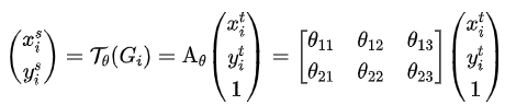
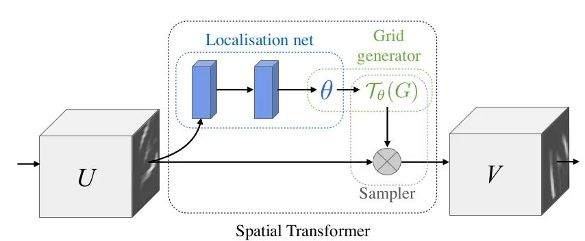
In this paper, STN module is proposed to explicitly implant spatial transformation into the network, so as to improve the invariance of rotation, translation and scale of the network. It can be understood as "alignment" operation. The structure of STN is shown in the figure above. Each STN module is composed of localization net, grid generator and Sampler. Localization net is used to learn and obtain the parameters of spatial transformation, which is the parameter in the above formula θ Six parameters. Grid generator is used for coordinate mapping. The Sampler is used for pixel acquisition by bilinear interpolation.
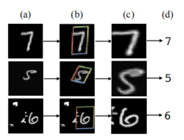
The meaning of STN is that it can correct the original image into the ideal image desired by the network, and the process is carried out in an unsupervised way, that is, the transformation parameters are obtained by spontaneous learning without labeling information. The module is an independent module that can be inserted anywhere on CNN. Meet the inventory requirements of this "plug-in".
Core code:
class SpatialTransformer(nn.Module):
    def __init__(self, spatial_dims):
        super(SpatialTransformer, self).__init__()
        self._h, self._w = spatial_dims
        self.fc1 = nn.Linear(32*4*4, 1024) # It can be set according to your own network parameters
        self.fc2 = nn.Linear(1024, 6)

    def forward(self, x):
        batch_images = x #Save a copy of the original data
        x = x.view(-1, 32*4*4)
        # Six parameters are learned by using FC structure
        x = self.fc1(x)
        x = self.fc2(x)
        x = x.view(-1, 2,3) # 2x3
        # Using affine_grid generates sampling points
        affine_grid_points = F.affine_grid(x, torch.Size((x.size(0), self._in_ch, self._h, self._w)))
        # Apply sample points to raw data
        rois = F.grid_sample(batch_images, affine_grid_points)
        return rois, affine_grid_points
2 ASPP
Full name of plug-in: atrus spatial pyramid pooling
From the paper: deep lab: semantic image segmentation with deep revolutionary networks, Atlas conv
Paper link: https://arxiv.org/pdf/1606.00915.pdf
Core resolution:
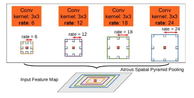
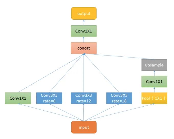
This plug-in is a spatial pyramid pooling module with hole convolution. It is mainly proposed to improve the receptive field of the network and introduce multi-scale information. We know that for semantic segmentation networks, we usually face images with large resolution, which requires our network to have enough receptive fields to cover the target object. For CNN networks, the receptive field is basically obtained by stacking the convolution layer and down sampling. This module can control the receptive field without changing the size of the feature map, which is conducive to extracting multi-scale information. rate controls the size of the receptive field. The larger r is, the larger the receptive field is.
ASPP mainly includes the following parts: 1 A global average pooling layer obtains the image level feature, performs 1X1 convolution, and bilinear interpolation to the original size; 2. One 1X1 convolution layer and three 3X3 cavity convolutions; 3. Concatenate the features of five different scales in the channel dimension, and then send them to 1X1 convolution for fusion output.
Core code:
class ASPP(nn.Module):
    def __init__(self, in_channel=512, depth=256):
        super(ASPP,self).__init__()
        self.mean = nn.AdaptiveAvgPool2d((1, 1))
        self.conv = nn.Conv2d(in_channel, depth, 1, 1)
        self.atrous_block1 = nn.Conv2d(in_channel, depth, 1, 1)
        # Convolution of different void rates
        self.atrous_block6 = nn.Conv2d(in_channel, depth, 3, 1, padding=6, dilation=6)
        self.atrous_block12 = nn.Conv2d(in_channel, depth, 3, 1, padding=12, dilation=12)
        self.atrous_block18 = nn.Conv2d(in_channel, depth, 3, 1, padding=18, dilation=18)
        self.conv_1x1_output = nn.Conv2d(depth * 5, depth, 1, 1)

    def forward(self, x):
        size = x.shape[2:]
     # Pooled branch
        image_features = self.mean(x)
        image_features = self.conv(image_features)
        image_features = F.upsample(image_features, size=size, mode='bilinear')
     # Convolution of different void rates
        atrous_block1 = self.atrous_block1(x)
        atrous_block6 = self.atrous_block6(x)
        atrous_block12 = self.atrous_block12(x)
        atrous_block18 = self.atrous_block18(x)
        # Combine the characteristics of all scales
     x = torch.cat([image_features, atrous_block1, atrous_block6,atrous_block12, atrous_block18], dim=1)
        # Fusion feature output using 1X1 convolution
        x = self.conv_1x1_output(x)
        return net
3 Non-local
From paper: non local neural networks
Paper link: https://arxiv.org/abs/1711.07971
Core resolution:
Non local is an attention mechanism and a module that is easy to implant and integrate. Local is mainly for the receptive field. Take the convolution operation and pooling operation in CNN as an example. The size of its receptive field is the size of the convolution kernel, and we often stack the convolution layer of 3X3. It only considers the local area and is all local operation. The difference is that the receptive field of non local operation can be large, which can be a global region rather than a local region. Capturing long-range dependencies, that is, how to establish the relationship between two pixels with a certain distance on the image, is an attention mechanism. The so-called attention mechanism is to use the network to generate salience map. Attention corresponds to the significant area, which needs the focus of the network.
-
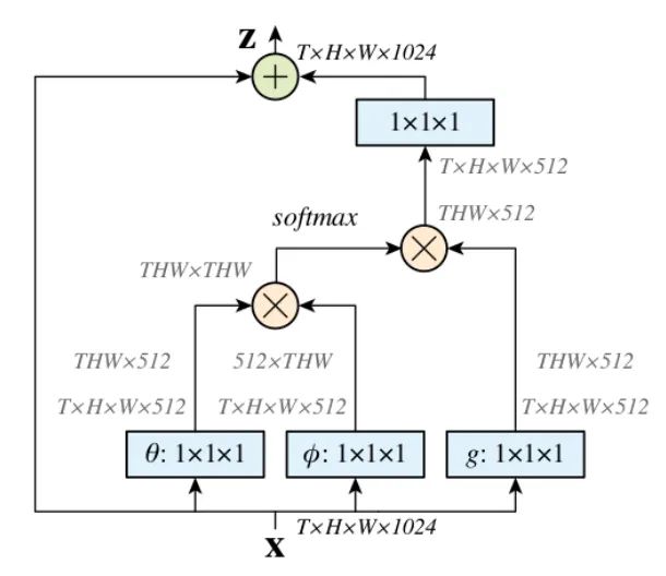
Firstly, the input characteristic map is convoluted by 1X1 to compress the number of channels and obtain θ,
 , g characteristics.
 -
Through reshape operation, transform the dimensions of the three features, and then θ,
The matrix multiplication operation is carried out to obtain a similar covariance matrix. This step is to calculate the autocorrelation in the feature, that is, to obtain the relationship between each pixel in each frame and all pixels in all other frames. -
Then perform Softmax operation on the autocorrelation features to obtain weights of 0 ~ 1. Here is the self attention coefficient we need.
-
Finally, multiply the attention coefficient back to the characteristic matrix g and add it to the residual of the original input feature map X for output.
Here, let's take a simple example and assume that g is (we don't consider the batch and channel dimensions for the time being):
g = torch.tensor([[1, 2], [3, 4]).view(-1, 1).float()
θ For:
theta = torch.tensor([2, 4, 6, 8]).view(-1, 1)
For:
phi = torch.tensor([7, 5, 3, 1]).view(1, -1)
So, θ andThe matrix is multiplied as follows:
tensor([[14., 10., 6., 2.], [28., 20., 12., 4.], [42., 30., 18., 6.], [56., 40., 24., 8.]])
After entering softmax(dim=-1), each line represents the importance of the elements in g. the value in front of each line is relatively large. Therefore, I hope to pay more attention to the elements in front of G, that is, 1 is more important. Alternatively, the attention matrix represents the dependence of each element in G on other elements.
tensor([[9.8168e-01, 1.7980e-02, 3.2932e-04, 6.0317e-06], [9.9966e-01, 3.3535e-04, 1.1250e-07, 3.7739e-11], [9.9999e-01, 6.1442e-06, 3.7751e-11, 2.3195e-16], [1.0000e+00, 1.1254e-07, 1.2664e-14, 1.4252e-21]])
After attention is applied, the overall value is close to the value in the original g to 1:
tensor([[1.0187, 1.0003], [1.0000, 1.0000]])
Core code:
class NonLocal(nn.Module):
    def __init__(self, channel):
        super(NonLocalBlock, self).__init__()
        self.inter_channel = channel // 2
        self.conv_phi = nn.Conv2d(channel, self.inter_channel, 1, 1,0, False)
        self.conv_theta = nn.Conv2d(channel, self.inter_channel, 1, 1,0, False)
        self.conv_g = nn.Conv2d(channel, self.inter_channel, 1, 1, 0, False)
        self.softmax = nn.Softmax(dim=1)
        self.conv_mask = nn.Conv2d(self.inter_channel, channel, 1, 1, 0, False)

    def forward(self, x):
        # [N, C, H , W]
        b, c, h, w = x.size()
        # Obtain the phi feature with the dimension [N, C/2, H * W]. Note that the batch and channel dimensions should be retained, which is carried out on HW
        x_phi = self.conv_phi(x).view(b, c, -1)
        # Get theta feature with dimension [N, H * W, C/2]
        x_theta = self.conv_theta(x).view(b, c, -1).permute(0, 2, 1).contiguous()
        # Obtain g feature with dimension [N, H * W, C/2]
        x_g = self.conv_g(x).view(b, c, -1).permute(0, 2, 1).contiguous()
        # Matrix multiplication of phi and theta, [N, H * W, H * W]
        mul_theta_phi = torch.matmul(x_theta, x_phi)
        # softmax pulled between 0 and 1
        mul_theta_phi = self.softmax(mul_theta_phi)
        # Matrix multiplication with g feature, [N, H * W, C/2]
        mul_theta_phi_g = torch.matmul(mul_theta_phi, x_g)
        # [N, C/2, H, W]
        mul_theta_phi_g = mul_theta_phi_g.permute(0, 2, 1).contiguous().view(b, self.inter_channel, h, w)
        # Number of 1X1 convolution expansion channels
        mask = self.conv_mask(mul_theta_phi_g)
        out = mask + x # Residual connection
        return out
4 SE
From the paper: squeeze and exception networks
Paper link: https://arxiv.org/pdf/1709.01507.pdf
Core resolution:
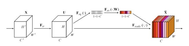
This article is the champion work of the last ImageNet competition. You will see it in many classic network structures, such as Mobilenet v3. It is actually a channel attention mechanism. Due to the existence of feature compression and FC, the captured channel attention features have global information. This paper proposes a new structural unit - "squeeze and exception (SE)" module, which can adaptively adjust the characteristic response value of each channel and model the internal dependency between channels. There are the following steps:
-
Squeeze: feature compression along the spatial dimension, turning each two-dimensional feature channel into a number, which is a global receptive field.
-
Exception: each feature channel generates a weight to represent the importance of the feature channel.
-
Reweight: regard the weight of the output of the exception as the importance of each feature channel and act on each channel by multiplying.
Core code:
class SE_Block(nn.Module):
    def __init__(self, ch_in, reduction=16):
        super(SE_Block, self).__init__()
        self.avg_pool = nn.AdaptiveAvgPool2d(1)  # Global adaptive pooling
        self.fc = nn.Sequential(
            nn.Linear(ch_in, ch_in // reduction, bias=False),
            nn.ReLU(inplace=True),
            nn.Linear(ch_in // reduction, ch_in, bias=False),
            nn.Sigmoid()
        )

    def forward(self, x):
        b, c, _, _ = x.size()
        y = self.avg_pool(x).view(b, c) # squeeze operation
        y = self.fc(y).view(b, c, 1, 1) # FC obtains the channel attention weight with global information
        return x * y.expand_as(x) # Attention acts on every channel
5 CBAM
From the paper: CBAM: Revolutionary block attention module
Paper link: https://openaccess.thecvf.com/content_ECCV_2018/papers/Sanghyun_Woo_Convolutional_Block_Attention_ECCV_2018_paper.pdf
Core resolution:
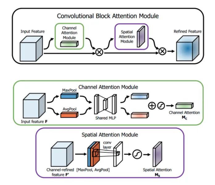
SENet obtains the attention weight on the channel of the feature map, and then multiplies it with the original feature map. This article points out that this attention method only focuses on which layers at the channel level will have stronger feedback ability, but it can not reflect attention in the spatial dimension. CBAM, as the highlight of this paper, applies attention to both channel and spatial dimensions. Like SE Module, CBAM can be embedded in most mainstream networks and can improve the feature extraction ability of the model without significantly increasing the amount of calculation and parameters.
Channel attention: as shown in the figure above, the input is an H × W × For the feature F of C, we first enter the global average pooling and maximum pooling of two spaces to obtain two 1 × one × Channel description of C. Then they are sent into a two-layer neural network. The number of neurons in the first layer is C/r, the activation function is Relu, and the number of neurons in the second layer is C. Note that this two-layer neural network is shared. Then, after adding the two features, the weight coefficient Mc is obtained through a Sigmoid activation function. Finally, the new scaled feature can be obtained by multiplying the weight coefficient with the original feature F. Pseudo code:
def forward(self, x):
    # Using FC to obtain global information is essentially the same as the matrix multiplication of non local
    avg_out = self.fc2(self.relu1(self.fc1(self.avg_pool(x))))
    max_out = self.fc2(self.relu1(self.fc1(self.max_pool(x))))
    out = avg_out + max_out
    return self.sigmoid(out)
Spatial attention: similar to channel attention, given an H × W × For the characteristic F 'of C, we first carry out the average pooling and maximum pooling of one channel dimension to obtain two H × W × 1, and splice the two descriptions together according to the channel. Then, after a 7 × 7, the activation function is Sigmoid, and the weight coefficient Ms is obtained. Finally, the new scaled feature can be obtained by multiplying the weight coefficient and the feature F '. Pseudo code:
def forward(self, x):
    # Here we use pooling to obtain global information
    avg_out = torch.mean(x, dim=1, keepdim=True)
    max_out, _ = torch.max(x, dim=1, keepdim=True)
    x = torch.cat([avg_out, max_out], dim=1)
    x = self.conv1(x)
    return self.sigmoid(x)
6 DCN v1&v2
Full name of plug-in: deformable revolutionary
From paper:
v1: [Deformable Convolutional Networks]
https://arxiv.org/pdf/1703.06211.pdf
v2: [Deformable ConvNets v2: More Deformable, Better Results]
https://arxiv.org/pdf/1811.11168.pdf
Core resolution:
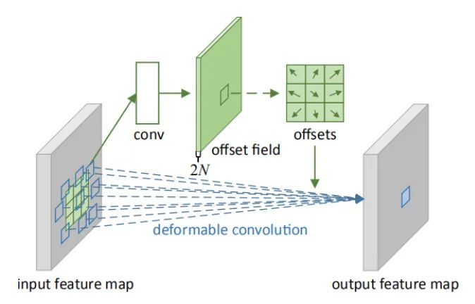
Deformation convolution can be regarded as deformation + convolution, so it can be used as a plug-in. In the major mainstream detection networks, deformation convolution is really a rising point artifact, and there are many online interpretations. Compared with the traditional fixed window convolution, deformation convolution can effectively deal with geometry, because its "local receptive field" is learnable and oriented to the whole graph. This paper also proposes deformable ROI pooling. Both methods are spatial sampling locations with additional offsets. They do not need additional supervision, but are self-monitoring processes.
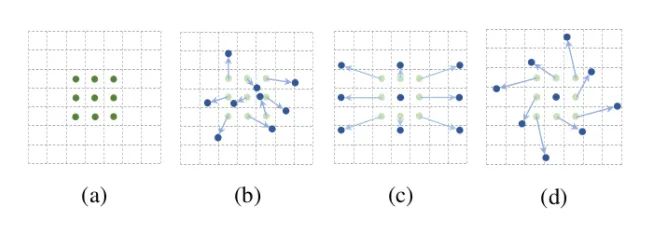
As shown in the above figure, a is different convolution, b is deformation convolution, and the dark point is the actual sampling position of convolution kernel, which is offset from the "standard" position. c and d are the special forms of deformation convolution, in which c is the common hole convolution, d is the convolution with learning rotation characteristics, and also has the ability to improve the receptive field.
Deformation convolution is very similar to STN process. STN uses the network to learn six parameters of spatial transformation and transform the feature map as a whole, in order to increase the ability of the network to extract deformation. DCN uses the network learning number to set the offset of the whole graph, which is more "comprehensive" than the deformation of STN. STN is affine transformation and DCN is arbitrary transformation. The formula is not pasted. You can directly see the code implementation process.
Deformable convolution has two versions: V1 and V2. V2 is improved on the basis of v2. In addition to sampling offset, it also increases sampling weight. V2 believes that 3X3 sampling points should also have different degrees of importance, so this processing method has more flexibility and fitting ability.
Core code:
def forward(self, x):
    # Learn the offset, including x and Y directions. Note that each pixel in each channel has an offset of x and y
    offset = self.p_conv(x)
    if self.v2: # In V2, an additional weight coefficient will be learned, which will be pulled between 0 and 1 through sigmoid
        m = torch.sigmoid(self.m_conv(x))
    # Use offset to interpolate x to obtain the offset x_offset
    x_offset = self.interpolate(x,offset)
    if self.v2: # When V2, the weight coefficient is applied to the feature map
        m = m.contiguous().permute(0, 2, 3, 1)
        m = m.unsqueeze(dim=1)
        m = torch.cat([m for _ in range(x_offset.size(1))], dim=1)
        x_offset *= m
    out = self.conv(x_offset) # After the action of offset, the standard convolution process is carried out
    return out
7 CoordConv
From the paper: an intriguing failing of revolutionary neural networks and the coordconv solution
Paper link: https://arxiv.org/pdf/1807.03247.pdf
Core resolution:
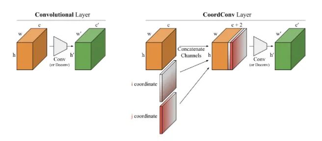
You can see it in Solo semantic segmentation algorithm and Yolov5. Starting from several small experiments, this paper explores the ability of convolution network in coordinate transformation. That is, it cannot convert the spatial representation into coordinates in Cartesian space. As shown in the figure below, we input (i, j) coordinates into a network and ask it to output a 64 × 64, and draw a square or a pixel at the coordinates, but the network can not be completed on the test set. Although this task is what we humans think is extremely simple. The reason is that when convolution is applied to the input as a local and shared weight filter, it does not know where each filter is and cannot capture the location information. So we can help convolution and let it know the location of the filter. You only need to add two channels to the input, one is the i coordinate and the other is the j coordinate. The specific method is shown in the figure above. Two channels are added before feeding into the filter. In this way, the network has the ability of spatial location information. Isn't it amazing? You can randomly use this pendant in tasks such as classification, segmentation and detection.
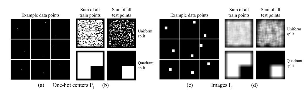
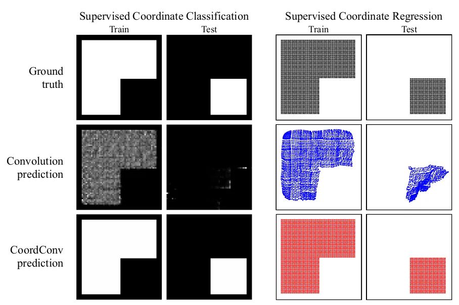
As shown in the first group of pictures above, in the task of generating images according to coordinate values, the training set is very good and the test set is a mess. The second group of pictures can easily complete the task after adding CoordConv, which can be seen that it increases the ability of CNN's spatial perception.
Core code:
ins_feat = x # Current instance feature tensor
# Generates a linear value from - 1 to 1
x_range = torch.linspace(-1, 1, ins_feat.shape[-1], device=ins_feat.device)
y_range = torch.linspace(-1, 1, ins_feat.shape[-2], device=ins_feat.device)
y, x = torch.meshgrid(y_range, x_range) # Generate 2D coordinate grid
y = y.expand([ins_feat.shape[0], 1, -1, -1]) # Extended to and ins_feat same dimension
x = x.expand([ins_feat.shape[0], 1, -1, -1])
coord_feat = torch.cat([x, y], 1) # Location features
ins_feat = torch.cat([ins_feat, coord_feat], 1) # Concatate is used as the input of the next convolution
8 Ghost
Full name of plug-in: Ghost module
From the paper: GhostNet: more features from cheapoperations
Paper link: https://arxiv.org/pdf/1911.11907.pdf
Core resolution:
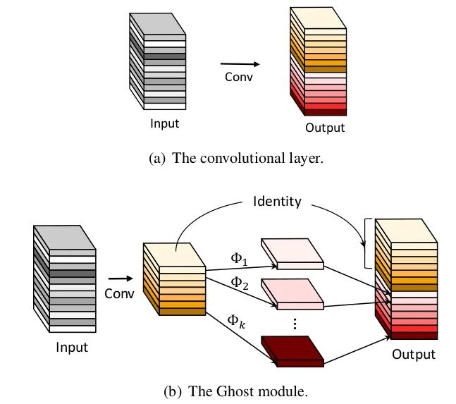
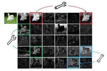
In the classification task of ImageNet, GhostNet has a Top-1 accuracy rate of 75.7% under the condition of similar calculation, which is higher than 75.2% of MobileNetV3. Its main innovation is the Ghost module. In CNN model, there is a lot of redundancy in feature map, which is of course very important and necessary. As shown in the figure below, the characteristic diagrams marked "small wrench" have redundant characteristic diagrams. So can we reduce the number of convolution channels, and then use some kind of transformation to generate redundant characteristic graphs? In fact, this is the idea of GhostNet.
Starting from the problem of feature graph redundancy, this paper proposes a structure - Ghost Module, which can generate a large number of feature graphs only through a small amount of calculation (called soap operations in the paper). The soap operations are linear transformation, which is realized by convolution operation in this paper. The specific process is as follows:
-
A smaller number of convolution operations than the original are used. For example, 64 convolution cores are normally used, and 32 convolution cores are used here, reducing the amount of computation by half.
-
Using depth separation convolution, redundant features are transformed from the feature map generated above.
-
The feature map obtained in the above two steps is concat output and sent to subsequent links.
Core code:
class GhostModule(nn.Module):
    def __init__(self, inp, oup, kernel_size=1, ratio=2, dw_size=3, stride=1, relu=True):
        super(GhostModule, self).__init__()
        self.oup = oup
        init_channels = math.ceil(oup / ratio)
        new_channels = init_channels*(ratio-1)

        self.primary_conv = nn.Sequential(
            nn.Conv2d(inp, init_channels, kernel_size, stride, kernel_size//2, bias=False),
            nn.BatchNorm2d(init_channels),
            nn.ReLU(inplace=True) if relu else nn.Sequential(), )
  # In the soap operation, pay attention to the use of packet convolution for channel separation
        self.cheap_operation = nn.Sequential(
            nn.Conv2d(init_channels, new_channels, dw_size, 1, dw_size//2, groups=init_channels, bias=False),
            nn.BatchNorm2d(new_channels),
            nn.ReLU(inplace=True) if relu else nn.Sequential(),)

    def forward(self, x):
        x1 = self.primary_conv(x)  #Main convolution operation
        x2 = self.cheap_operation(x1) # Soap transform operation
        out = torch.cat([x1,x2], dim=1) # The two are cat together
        return out[:,:self.oup,:,:]
9 BlurPool
From the paper: making revolutionary networks shift invariant again
Paper link: https://arxiv.org/abs/1904.11486
Core resolution:
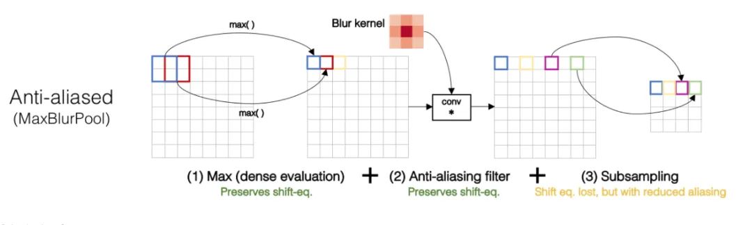
We all know that the convolution operation based on sliding window is translation invariant, so it is also assumed that CNN network is translation invariant or equivariant by default. Is this really the case? Practice has found that CNN network is really sensitive. As long as the input picture is slightly changed by one pixel or shifted by one pixel, the output of CNN will change greatly, and even the prediction will be wrong. This is very not robust. In general, we use data enhancement to obtain the so-called invariance. It is found that the fundamental reason for the degradation of invariance lies in down sampling. Whether it is max pool or Average Pool, or convolution operation with stripe > 1, as long as it involves down sampling with step size greater than 1, it will lead to the loss of translation invariance. The specific example is shown in the figure below. If you only translate one pixel, the result of max pool is very different.
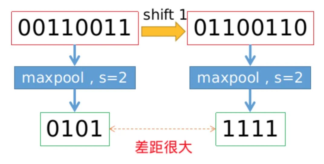
In order to maintain translation invariance, low-pass filtering can be performed before down sampling. The traditional max pool can be divided into two parts: MAX + down sampling with stripe = 1. Therefore, the author proposed MaxBlurPool = max + blur + down sampling to replace the original max pool. Experiments show that although this operation can not completely solve the loss of translation invariance, it can be alleviated to a great extent.
Core code:
class BlurPool(nn.Module):
    def __init__(self, channels, pad_type='reflect', filt_size=4, stride=2, pad_off=0):
        super(BlurPool, self).__init__()
        self.filt_size = filt_size
        self.pad_off = pad_off
        self.pad_sizes = [int(1.*(filt_size-1)/2), int(np.ceil(1.*(filt_size-1)/2)), int(1.*(filt_size-1)/2), int(np.ceil(1.*(filt_size-1)/2))]
        self.pad_sizes = [pad_size+pad_off for pad_size in self.pad_sizes]
        self.stride = stride
        self.off = int((self.stride-1)/2.)
        self.channels = channels
    # Define a series of Gaussian kernels
        if(self.filt_size==1):
            a = np.array([1.,])
        elif(self.filt_size==2):
            a = np.array([1., 1.])
        elif(self.filt_size==3):
            a = np.array([1., 2., 1.])
        elif(self.filt_size==4):
            a = np.array([1., 3., 3., 1.])
        elif(self.filt_size==5):
            a = np.array([1., 4., 6., 4., 1.])
        elif(self.filt_size==6):
            a = np.array([1., 5., 10., 10., 5., 1.])
        elif(self.filt_size==7):
            a = np.array([1., 6., 15., 20., 15., 6., 1.])

        filt = torch.Tensor(a[:,None]*a[None,:])
        filt = filt/torch.sum(filt) # Normalization operation ensures that the total amount of information remains unchanged after the feature passes through blur
        # The parameters of non grad operation are stored in buffer
        self.register_buffer('filt', filt[None,None,:,:].repeat((self.channels,1,1,1)))
        self.pad = get_pad_layer(pad_type)(self.pad_sizes)

    def forward(self, inp):
        if(self.filt_size==1):
            if(self.pad_off==0):
                return inp[:,:,::self.stride,::self.stride]
            else:
                return self.pad(inp)[:,:,::self.stride,::self.stride]
        else:
            # Using conv2d + stripe with fixed parameters to realize bluepool
            return F.conv2d(self.pad(inp), self.filt, stride=self.stride, groups=inp.shape[1])
10 RFB
Full name of plug-in: Receptive Field Block
From the paper: Receptive Field Block Net for Accurate and Fast Object Detection
Paper link: https://arxiv.org/abs/1711.07767
Core resolution:
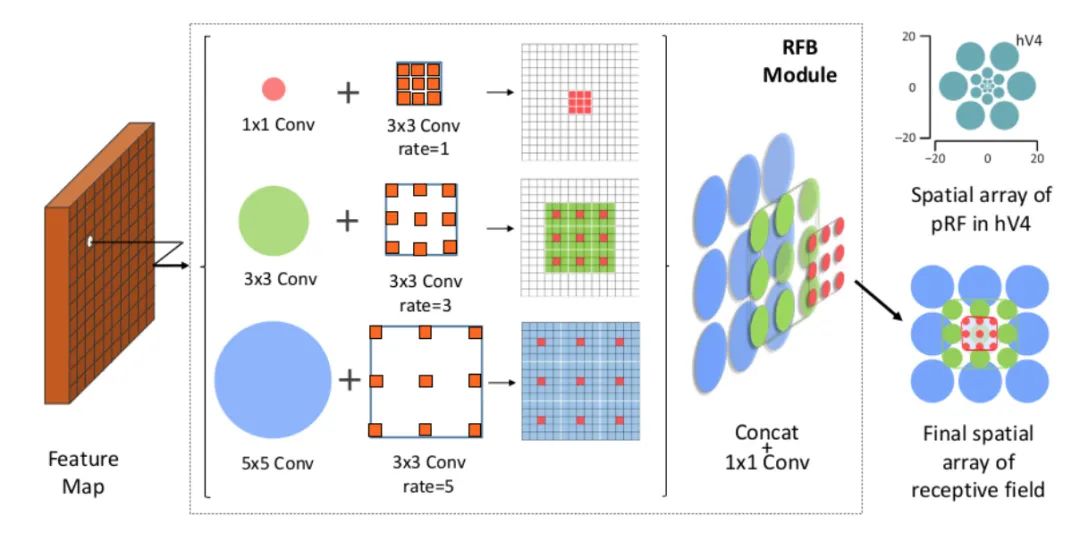
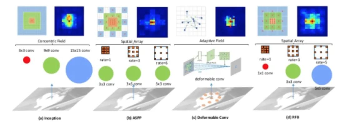
It is found that the target area should be as close to the center of the receptive field as possible, which will help to improve the robustness of the model to small-scale spatial displacement. Therefore, inspired by the RF structure of human vision, this paper proposes the receptive field module (RFB), which strengthens the ability of deep features learned by CNN model and makes the detection model more accurate. RFB can be embedded into most networks as a general module. The following figure shows the difference between it and inception, ASPP and DCN, which can be regarded as the combination of inception+ASPP.
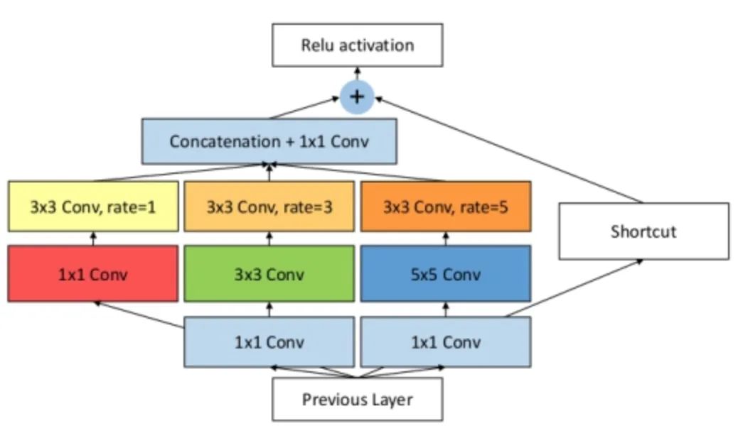
The specific implementation is shown in the figure below. In fact, it is similar to ASPP, but convolution cores of different sizes are used as the pre operation of void convolution.
Core code:
class RFB(nn.Module):
    def __init__(self, in_planes, out_planes, stride=1, scale = 0.1, visual = 1):
        super(RFB, self).__init__()
        self.scale = scale
        self.out_channels = out_planes
        inter_planes = in_planes // 8
        # Branch 0:1X1 convolution + 3X3 convolution
        self.branch0 = nn.Sequential(conv_bn_relu(in_planes, 2*inter_planes, 1, stride),
                conv_bn_relu(2*inter_planes, 2*inter_planes, 3, 1, visual, visual, False))
        # Branch 1:1X1 convolution + 3X3 convolution + void convolution
        self.branch1 = nn.Sequential(conv_bn_relu(in_planes, inter_planes, 1, 1),
                conv_bn_relu(inter_planes, 2*inter_planes, (3,3), stride, (1,1)),
                conv_bn_relu(2*inter_planes, 2*inter_planes, 3, 1, visual+1,visual+1,False))
        # Branch 2: 1X1 convolution + 3X3 convolution * 3 instead of 5X5 convolution + void convolution
        self.branch2 = nn.Sequential(conv_bn_relu(in_planes, inter_planes, 1, 1),
                conv_bn_relu(inter_planes, (inter_planes//2)*3, 3, 1, 1),
                conv_bn_relu((inter_planes//2)*3, 2*inter_planes, 3, stride, 1),
                conv_bn_relu(2*inter_planes, 2*inter_planes, 3, 1, 2*visual+1, 2*visual+1,False)  )
        self.ConvLinear = conv_bn_relu(6*inter_planes, out_planes, 1, 1, False)
        self.shortcut = conv_bn_relu(in_planes, out_planes, 1, stride, relu=False)
        self.relu = nn.ReLU(inplace=False)
    def forward(self,x):
        x0 = self.branch0(x)
        x1 = self.branch1(x)
        x2 = self.branch2(x)
    # Scale fusion
        out = torch.cat((x0,x1,x2),1)
        # 1X1 convolution
        out = self.ConvLinear(out)
        short = self.shortcut(x)
        out = out*self.scale + short
        out = self.relu(out)
        return out
11 ASFF
Full name of plug-in: adaptive spatial feature fusion
From the paper: adaptive spatial feature fusion learning spatial fusion for single shot object detection
Paper link: https://arxiv.org/abs/1911.09516v1
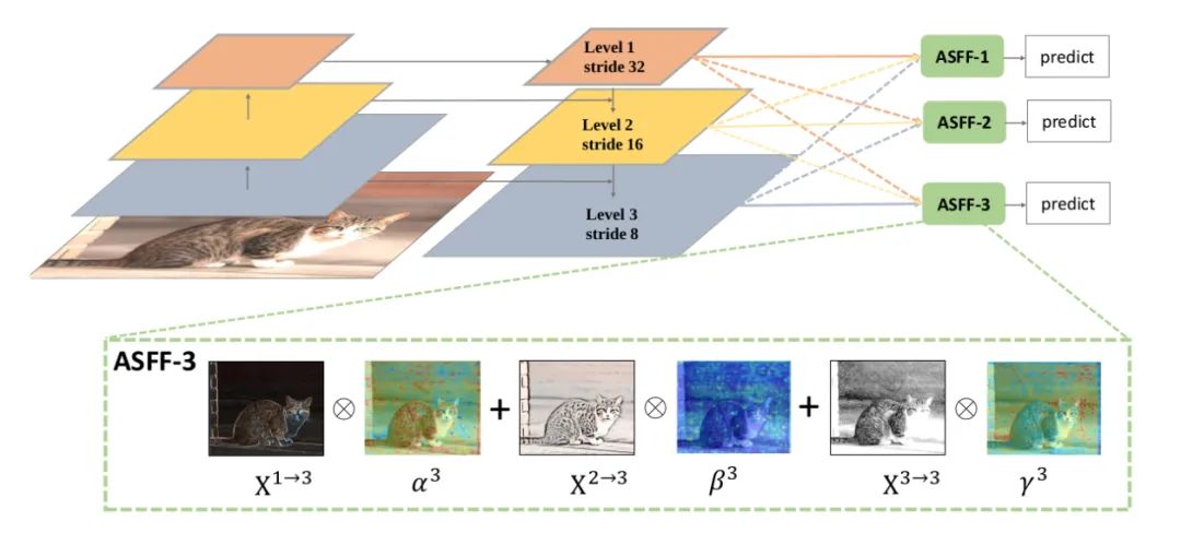
Core resolution:
In this paper, we think that the multi-level feature fusion and the multi-level feature fusion can make full use of the low-level feature fusion, that is, the multi-level feature fusion can not make full use of the low-level feature fusion. The characteristic diagram output by FPN is processed in the following two parts:
Feature Resizing: element wise fusion cannot be performed due to different scales of feature map, so resizing is required. For up sampling: firstly, 1X1 convolution is used for channel compression, and then interpolation is used to up sample the feature map. For 1 / 2 down sampling: 3X3 convolution with stripe = 2 is used for channel compression and characteristic image reduction at the same time. For 1 / 4 down sampling: insert maxpooling with stripe = 2 before the convolution of 3X3 with stripe = 2.
Adaptive Fusion: Adaptive Fusion of feature map. The formula is as follows:
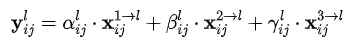
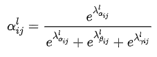
Where x, n → l represents the feature vector at the position (i, j), which comes from the N feature map and goes through the above resize to l scale. Alpha. Beta and gamma are spatial attention weights, which are processed by softmax as follows:
Code analysis:
class ASFF(nn.Module):
    def __init__(self, level, rfb=False):
        super(ASFF, self).__init__()
        self.level = level
        # Input the channels of the three feature layers and modify them according to the actual situation
        self.dim = [512, 256, 256]
        self.inter_dim = self.dim[self.level]
        # The number of output channels of the three at each level shall be consistent
        if level==0:
            self.stride_level_1 = conv_bn_relu(self.dim[1], self.inter_dim, 3, 2)
            self.stride_level_2 = conv_bn_relu(self.dim[2], self.inter_dim, 3, 2)
            self.expand = conv_bn_relu(self.inter_dim, 1024, 3, 1)
        elif level==1:
            self.compress_level_0 = conv_bn_relu(self.dim[0], self.inter_dim, 1, 1)
            self.stride_level_2 = conv_bn_relu(self.dim[2], self.inter_dim, 3, 2)
            self.expand = conv_bn_relu(self.inter_dim, 512, 3, 1)
        elif level==2:
            self.compress_level_0 = conv_bn_relu(self.dim[0], self.inter_dim, 1, 1)
            if self.dim[1] != self.dim[2]:
                self.compress_level_1 = conv_bn_relu(self.dim[1], self.inter_dim, 1, 1)
            self.expand = add_conv(self.inter_dim, 256, 3, 1)
        compress_c = 8 if rfb else 16
        self.weight_level_0 = conv_bn_relu(self.inter_dim, compress_c, 1, 1)
        self.weight_level_1 = conv_bn_relu(self.inter_dim, compress_c, 1, 1)
        self.weight_level_2 = conv_bn_relu(self.inter_dim, compress_c, 1, 1)

        self.weight_levels = nn.Conv2d(compress_c*3, 3, 1, 1, 0)

  # Scale level_ 0 < level_ 1 < level_ two
    def forward(self, x_level_0, x_level_1, x_level_2):
        # Feature Resizing process
        if self.level==0:
            level_0_resized = x_level_0
            level_1_resized = self.stride_level_1(x_level_1)
            level_2_downsampled_inter =F.max_pool2d(x_level_2, 3, stride=2, padding=1)
            level_2_resized = self.stride_level_2(level_2_downsampled_inter)
        elif self.level==1:
            level_0_compressed = self.compress_level_0(x_level_0)
            level_0_resized =F.interpolate(level_0_compressed, 2, mode='nearest')
            level_1_resized =x_level_1
            level_2_resized =self.stride_level_2(x_level_2)
        elif self.level==2:
            level_0_compressed = self.compress_level_0(x_level_0)
            level_0_resized =F.interpolate(level_0_compressed, 4, mode='nearest')
            if self.dim[1] != self.dim[2]:
                level_1_compressed = self.compress_level_1(x_level_1)
                level_1_resized = F.interpolate(level_1_compressed, 2, mode='nearest')
            else:
                level_1_resized =F.interpolate(x_level_1, 2, mode='nearest')
            level_2_resized =x_level_2
    # Fusion weight also comes from e-learning
        level_0_weight_v = self.weight_level_0(level_0_resized)
        level_1_weight_v = self.weight_level_1(level_1_resized)
        level_2_weight_v = self.weight_level_2(level_2_resized)
        levels_weight_v = torch.cat((level_0_weight_v, level_1_weight_v,
                                     level_2_weight_v),1)
        levels_weight = self.weight_levels(levels_weight_v)
        levels_weight = F.softmax(levels_weight, dim=1)   # alpha generation
    # Adaptive fusion
        fused_out_reduced = level_0_resized * levels_weight[:,0:1,:,:]+\
                            level_1_resized * levels_weight[:,1:2,:,:]+\
                            level_2_resized * levels_weight[:,2:,:,:]

        out = self.expand(fused_out_reduced)
        return out
epilogue
This article reviews the exquisite and practical CNN plug-ins in recent years. I hope you can learn and use them flexibly and use them in your own practical projects.