Note: this blog is a summary of Mr. Li Hang's notes on statistical learning methods. Many contents in the blog are extracted from Mr. Li Hang's Book Statistical learning methods, which is only for learning and communication.
Generation of decision tree
In the last blog Decision tree (I) -- Construction of decision tree In, we have described the feature selection in the three steps of decision tree. Today, we will first explain the generation of decision tree.
The basic idea of decision tree generation is to segment data sets. The specific approach is to try each feature and measure which feature will bring you the best results, and then segment the data set based on the optimal feature (since the optimal feature may have several values, we may also get multiple subsets). After the first partition, the data set is passed down to the next node of the branch of the tree. At this node, we can divide the data again. That is, we can use recursion to process data sets.
The algorithms of decision tree generation include ID3 and C4.5. Let's explain the ID3 algorithm first.
ID3
The core of ID3 algorithm is to apply the information gain criterion to select features on each node of the decision tree and construct the decision tree recursively.
Input: training data set D, feature set A, threshold ε
Output: decision tree T
(1) If all instances in D belong to the same class C k C_k Ck, then T is a single node tree, and the class C k C_k Ck , as the class mark of the node, returns T;
(2) If A = ∅ A=∅ A = ∅, then T is a single node tree, and the class with the largest number of instances in D C k C_k Ck , as the class mark of the node, returns T;
(3) Otherwise, calculate the information gain of each feature pair D in A and select the feature with the largest information gain A g A_g Ag;
(4) If A g A_g The information gain of Ag is less than the threshold ε, Then set T as a single node tree and the class with the largest number of instances in D C k C_k Ck , as the class mark of the node, returns T;
(5) Otherwise, yes A g A_g Every possible value of Ag + a i a_i ai, Yi A g = a i A_g=a_i Ag = ai , divides D into several non empty subsets D i D_i Di, will D i D_i The class with the largest number of instances in Di , is the most marked, constructs child nodes, forms a tree T from nodes and their child nodes, and returns t;
(6) For the ith child node, the D i D_i Di , is the training set A − { A g } A-\{A_g\} A − {Ag} is the feature set, and steps (1) ~ (5) are recursively called to obtain the subtree T i T_i Ti, return T i T_i Ti.
give an example
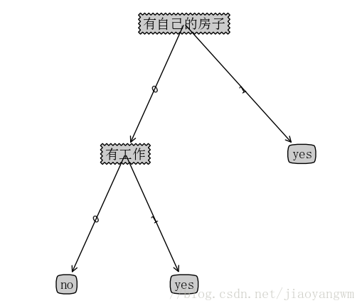
In fact, in the last blog, we calculated the information gain of each feature. We already know that the third feature (with its own house) has the largest information gain, so it is the root node of the decision tree; Then, there are two values for the feature: Yes or no, so we can divide the data set D into two subsets D yes D_ yes D is , and D no D_ no D no, then the dataset should be like this: (after selecting the best feature, we need to delete the label of the best feature and its value in the dataset)
D yes D_ yes D is:
| ID | Age | Have a job | Credit situation | category |
|---|---|---|---|---|
| 4 | youth | yes | commonly | yes |
| 8 | middle age | yes | good | yes |
| 9 | middle age | no | very nice | yes |
| 10 | middle age | no | very nice | yes |
| 11 | old age | no | very nice | yes |
| 12 | old age | no | good | yes |
According to the table, the categories with their own houses are yes, which meets the first item of the decision tree algorithm, so the return class label is yes.
D no D_ no D No:
| ID | Age | Have a job | Credit situation | category |
|---|---|---|---|---|
| 1 | youth | no | commonly | no |
| 2 | youth | no | good | no |
| 3 | youth | yes | good | yes |
| 5 | youth | no | commonly | no |
| 6 | middle age | no | commonly | no |
| 7 | middle age | no | good | no |
| 13 | old age | yes | good | yes |
| 14 | old age | yes | very nice | yes |
| 15 | old age | no | commonly | no |
subset D no D_ no D) if no, it needs to be calculated g ( D no , A ) g(D_; no, A) g(D, no, A) to compare which feature is more suitable for subset D no D_ no D is the root node of No. let's take you to calculate it briefly.
hypothesis
A
1
A_1
A1 = characteristic age,
A
2
A_2
A2 indicates that the features are,
A
3
A_3
A3 , indicates characteristic credit
g
(
D
no
,
A
1
)
=
H
(
D
no
)
−
H
(
D
no
,
A
1
)
=
−
6
9
l
o
g
2
6
9
−
3
9
l
o
g
2
3
9
−
[
4
9
(
−
3
4
l
o
g
2
3
4
−
1
4
l
o
g
2
1
4
)
+
2
9
∗
0
+
3
9
(
−
2
3
l
o
g
2
2
3
−
1
3
l
o
g
2
1
3
)
]
=
0.918
−
(
0.361
+
0
+
0.306
)
=
0.251
\begin{aligned} g(D no, a _1) & = H(D no) - H(D no, a _1) \ \ & = - \ frac {6} {9} log_ 2\frac{6}{9}-\frac{3}{9}log_ 2\frac{3}{9}-[\frac{4}{9}(-\frac{3}{4}log_2\frac{3}{4}-\frac{1}{4}log_2\frac{1}{4})+\frac{2}{9}*0+\frac{3}{9}(-\frac{2}{3}log_2\frac{2}{3}-\frac{1}{3}log_2\frac{1}{3})] \ &=0.918-(0.361+0+0.306) \ &=0.251 \end{aligned}
G (dno, A1) = H (dno) − H (dno, A1) = 96 − 93 log2 93 − [94 (− 43 log2 43 − 41 log2 41) + 92 * 0 + 93 (− 32 log2 32 − 31 log2 31)] = 0.918 − (0.361 + 0 + 0.306) = 0.251
Other features are the same.
code implementation
from math import log
import operator

def createDataSet():
    # data set
    dataSet=[[0, 0, 0, 0, 'no'],
            [0, 0, 0, 1, 'no'],
            [0, 1, 0, 1, 'yes'],
            [0, 1, 1, 0, 'yes'],
            [0, 0, 0, 0, 'no'],
            [1, 0, 0, 0, 'no'],
            [1, 0, 0, 1, 'no'],
            [1, 1, 1, 1, 'yes'],
            [1, 0, 1, 2, 'yes'],
            [1, 0, 1, 2, 'yes'],
            [2, 0, 1, 2, 'yes'],
            [2, 0, 1, 1, 'yes'],
            [2, 1, 0, 1, 'yes'],
            [2, 1, 0, 2, 'yes'],
            [2, 0, 0, 0, 'no']]
    #Classification properties
    labels=['Age','Have a job','Have your own house','Credit situation']
    #Return dataset and classification properties
    return dataSet,labels

#Shannon entropy (empirical entropy)
def calcShannonEnt(dataSet):
    #Number of data set rows
    numEntries=len(dataSet)
    #A dictionary that holds the number of occurrences of class labels
    labelCounts={}
    #Each group of eigenvectors is counted
    for featVec in dataSet:
        currentLabel=featVec[-1]                     #Class label
        if currentLabel not in labelCounts.keys():   #If the label is not put into the dictionary of statistical times, add it
            labelCounts[currentLabel]=0
        labelCounts[currentLabel]+=1

    shannonEnt=0.0
    #Computational empirical entropy
    for key in labelCounts:
        prob=float(labelCounts[key])/numEntries
        shannonEnt-=prob*log(prob,2)
    return shannonEnt                                #Return empirical entropy

#Split dataset
def splitDataSet(dataSet,axis,value):
    retDataSet=[]
    #Traversal dataset
    for featVec in dataSet:
        if featVec[axis]==value:
            #Remove axis feature
            reduceFeatVec=featVec[:axis]
            reduceFeatVec.extend(featVec[axis+1:])
            #Add eligible to the returned dataset
            retDataSet.append(reduceFeatVec)
    return retDataSet

#The class with the largest number of realistic instances
def majorityCnt(classList):
    classCount={}
    #Count the number of occurrences of each element in the classList
    for vote in classList:
        if vote not in classCount.keys():
            classCount[vote]=0
        classCount[vote]+=1
    #Sort in descending order according to the values of the dictionary
    sortedClassCount=sorted(classCount.items(),key=operator.itemgetter(1),reverse=True)
    return sortedClassCount[0][0]

#Select the optimal feature (based on information gain or information gain ratio)
def chooseBestFeatureToSplit(dataSet):
    #Number of features
    numFeatures = len(dataSet[0]) - 1
    baseEntropy = calcShannonEnt(dataSet)
    #information gain
    bestInfoGain = 0.0
    #Index value of optimal feature
    bestFeature = -1
    #Traverse all features
    for i in range(numFeatures):
        # Get the i th all features of dataSet
        featList = [example[i] for example in dataSet]
        #Create set set {}, elements cannot be repeated
        uniqueVals = set(featList)
        #Empirical conditional entropy
        newEntropy = 0.0
        #Calculate information gain
        for value in uniqueVals:
            #The subset of the subDataSet after partition
            subDataSet = splitDataSet(dataSet, i, value)
            prob = len(subDataSet) / float(len(dataSet))
            #The empirical conditional entropy is calculated according to the formula
            newEntropy += prob * calcShannonEnt((subDataSet))
        #information gain
        infoGain = baseEntropy - newEntropy
        #Print information gain for each feature
        print("The first%d The gain of each feature is%.3f" % (i, infoGain))
        #Select the feature with the largest information gain and store its index
        if (infoGain > bestInfoGain):
            bestInfoGain = infoGain
            bestFeature = i
    return bestFeature

#Create decision tree
def createTree(dataSet,labels,featLabels):
    #Read class label
    classList=[example[-1] for example in dataSet]
    #If all instances in D belong to the same class
    if classList.count(classList[0])==len(classList):
        return classList[0]
    #When all features are traversed, the class label with the most occurrences is returned
    if len(dataSet[0])==1:
        return majorityCnt(classList)
    #Select the optimal feature
    bestFeat=chooseBestFeatureToSplit(dataSet)
    #Optimal feature label
    bestFeatLabel=labels[bestFeat]
    featLabels.append(bestFeatLabel)
    #Label spanning tree based on optimal features
    myTree={bestFeatLabel:{}}
    #Delete used feature labels
    del(labels[bestFeat])
    #The attribute values of all optimal features in the training set are obtained
    featValues=[example[bestFeat] for example in dataSet]
    #Remove duplicate attribute values
    uniqueVls=set(featValues)
    #Traverse the features to create a decision tree
    for value in uniqueVls:
        myTree[bestFeatLabel][value]=createTree(splitDataSet(dataSet,bestFeat,value),
                                               labels,featLabels)
    return myTree

if __name__=='__main__':
    dataSet,labels=createDataSet()
    featLabels=[]
    myTree=createTree(dataSet,labels,featLabels)
    print(myTree)
The gain of the 0th feature is 0.083
 The gain of the first feature is 0.324
 The gain of the second feature is 0.420
 The gain of the third feature is 0.363
 The gain of the 0th feature is 0.252
 The gain of the first feature is 0.918
 The gain of the second feature is 0.474
{'Have your own house': {0: {'Have a job': {0: 'no', 1: 'yes'}}, 1: 'yes'}}
C4.5
C4.5 is very similar to ID3, but the information gain ratio is not used when selecting the optimal feature, so I won't repeat it here.
code implementation
For the implementation of C4.5 algorithm, please refer to ID3. Here I simply show the parts that need to be modified.
As we all know, the formula of information gain ratio is g R ( D , A ) = g ( D , A ) H A ( D ) g_R(D,A)=\frac{g(D,A)}{H_A(D)} gR (D,A)=HA (D)g(D,A). Let's simply calculate it here H A ( D ) H_A(D) HA(D)
We have calculated the information gain of the first feature before, and we will use it directly here.
g
(
D
,
A
1
)
=
0.083
g(D,A_1)=0.083
g(D,A1)=0.083
H
A
1
(
D
)
=
−
∑
i
=
1
n
∣
D
i
∣
∣
D
∣
l
o
g
2
∣
D
i
∣
∣
D
∣
=
−
5
15
l
o
g
2
5
15
−
5
15
l
o
g
2
5
15
−
5
15
l
o
g
2
5
15
=
−
l
o
g
2
5
15
=
1.585
\begin{aligned} H_{A_1}(D)&=-\sum_{i=1}^n\frac{|D_i|}{|D|}log_2\frac{|D_i|}{|D|} \\ &=-\frac{5}{15}log_2\frac{5}{15}-\frac{5}{15}log_2\frac{5}{15}-\frac{5}{15}log_2\frac{5}{15} \\ &=-log_2\frac{5}{15} \\ &=1.585 \end{aligned}
HA1(D)=−i=1∑n∣D∣∣Di∣log2∣D∣∣Di∣=−155log2155−155log2155−155log2155=−log2155=1.585
g
R
(
D
,
A
)
=
g
(
D
,
A
)
H
A
(
D
)
=
0.083
1.585
≈
0.052
g_R(D,A)=\frac{g(D,A)}{H_A(D)}=\frac{0.083}{1.585}≈0.052
gR(D,A)=HA(D)g(D,A)=1.5850.083≈0.052
The following calcAShannonEnt() function is the H A ( D ) H_A(D) Calculation of HA (D).
def calcAShannonEnt(dataSet,i):
    #Returns the number of rows in the dataset
    numEntries=len(dataSet)
    #Save a dictionary of the number of occurrences of each label
    labelCounts={}
    #Each group of eigenvectors is counted
    for featVec in dataSet:
        currentLabel=featVec[i]                     #Extract label information
        if currentLabel not in labelCounts.keys():   #If the label is not put into the dictionary of statistical times, add it
            labelCounts[currentLabel]=0
        labelCounts[currentLabel]+=1                 #label count

    shannonEnt=0.0                                   #Empirical entropy
    #Computational empirical entropy
    for key in labelCounts:
        prob=float(labelCounts[key])/numEntries      #Probability of selecting the label
        shannonEnt-=prob*log(prob,2)                 #Calculation by formula
    return shannonEnt
What needs to be changed next is the chooseBestFeatureToSplit() function, which mainly calculates the information gain g ( D , A ) g(D,A) g(D,A) and empirical entropy of feature A data set H A ( D ) H_A(D) Ratio between HA (D).
def chooseBestFeatureToSplit(dataSet):
    #Number of features
    numFeatures = len(dataSet[0]) - 1
    #Shannon entropy of counting data set
    baseEntropy = calcShannonEnt(dataSet)
    #information gain
    bestInfoGainRate = 0.0
    #Index value of optimal feature
    bestFeature = -1
    #Traverse all features
    for i in range(numFeatures):
        # Get the i th all features of dataSet
        featList = [example[i] for example in dataSet]
        #Create set set {}, elements cannot be repeated
        uniqueVals = set(featList)
        #Empirical conditional entropy
        newEntropy = 0.0
        #Calculate information gain
        for value in uniqueVals:
            #The subset of the subDataSet after partition
            subDataSet = splitDataSet(dataSet, i, value)
            #Calculate the probability of subsets
            prob = len(subDataSet) / float(len(dataSet))
            #The empirical conditional entropy is calculated according to the formula
            newEntropy += prob * calcShannonEnt((subDataSet))
        #information gain
        infoGain = baseEntropy - newEntropy
        if calcAShannonEnt(dataSet,i) == 0:
            continue
        #information gain
        infoGain = baseEntropy - newEntropy
        #print("gain ratio of feature% d is%. 3F"% (I, infogain))
        if calcAShannonEnt(dataSet,i) == 0:
            continue
        #print("gain ratio of feature% d is%. 3F"% (I, calcashannonenent (dataset, I)))
        #Information gain ratio
        infoGainRate = infoGain / calcAShannonEnt(dataSet,i)
        print("The first%d The gain ratio of each feature is%.3f" % (i, infoGainRate))
        #Calculate information gain
        if (infoGainRate > bestInfoGainRate):
            #Update the information gain to find the maximum information gain
            bestInfoGainRate = infoGainRate
            #Record the index value of the feature with the largest information gain
            bestFeature = i
            #Returns the index value of the feature with the maximum information gain
    return bestFeature
The gain ratio of the 0th feature is 0.052
 The gain ratio of the first feature is 0.352
 The gain ratio of the second feature is 0.433
 The gain ratio of the third feature is 0.232
 The gain ratio of the 0th feature is 0.164
 The gain ratio of the first feature is 1.000
 The gain ratio of the second feature is 0.340
{'Have your own house': {0: {'Have a job': {0: 'no', 1: 'yes'}}, 1: 'yes'}}
cart generation algorithm
cart model is divided into regression tree and classification tree, and only the classification tree is explained here.
The classification tree uses Gini index to select the optimal feature and determine the most binary segmentation point of the feature.
Gini index: in the classification problem, suppose there are k classes, and the probability that the sample points belong to class k is
p
k
p_k
pk, then the Gini index of the probability distribution is defined as
G
i
n
i
(
p
)
=
∑
k
=
1
K
p
k
(
1
−
p
k
)
=
1
−
∑
k
=
1
K
p
k
2
Gini(p)=\sum_{k=1}^Kp_k(1-p_k)=1-\sum_{k=1}^Kp_k^2
Gini(p)=k=1∑Kpk(1−pk)=1−k=1∑Kpk2
For class II classification problems, if the probability that the sample points belong to the first class is p, the Gini index of the probability distribution is
G
i
n
i
(
p
)
=
2
p
(
1
−
p
)
Gini(p)=2p(1-p)
Gini(p)=2p(1−p)
For a given sample set D, its Gini index is
G
i
n
i
(
D
)
=
1
−
∑
k
=
1
K
(
∣
C
k
∣
∣
D
∣
)
2
Gini(D)=1-\sum_{k=1}^K(\frac{|C_k|}{|D|})^2
Gini(D)=1−k=1∑K(∣D∣∣Ck∣)2
If the sample set D takes a possible value according to whether the feature a is divided into
D
1
D_1
D1 , and
D
2
D_2
D2 , two parts, i.e
D
1
=
{
(
x
,
y
)
∈
D
∣
A
(
x
)
=
a
}
,
D
2
=
D
−
D
1
D_1=\{(x,y)∈D|A(x)=a\}, \ D_2=D-D_1
D1={(x,y)∈D∣A(x)=a}, D2=D−D1
Then, under the condition of characteristic A, the Gini index of set D is defined as
G
i
n
i
(
D
,
A
)
=
∣
D
1
∣
∣
D
2
∣
G
i
n
i
(
D
1
)
+
∣
D
2
∣
∣
D
∣
G
i
n
i
(
D
2
)
Gini(D,A)=\frac{|D_1|}{|D_2|}Gini(D_1)+\frac{|D_2|}{|D|}Gini(D_2)
Gini(D,A)=∣D2∣∣D1∣Gini(D1)+∣D∣∣D2∣Gini(D2)
Note: Gini index Gini(D) represents the uncertainty of set D, and Gini index Gini(D,A) represents the uncertainty of set d after A=a.
generating algorithm
Input: training data set D, conditions for stopping calculation;
Output: CART decision tree
According to the training data set, starting from the root node, recursively perform the following operations on each node to construct a binary decision tree.
(1) Let the training data set of the node be D, and calculate the Gini index of the existing features to the data set. At this time, for each feature a, for which each value a may be obtained, D is divided into two parts according to whether the test of sample point A=a is "yes" or "no" D 1 D_1 D1 , and D 2 D_2 D2 , calculate the Gini index when A=a by using the last formula above.
(2) Among all possible features a and all their possible segmentation points a, the feature with the smallest Gini index and its corresponding segmentation point are selected as the optimal feature and optimal segmentation point. According to the optimal feature and optimal cut point, two sub nodes are generated from the current node, and the training data set is allocated to the two sub nodes according to the feature.
(3) Recursively call (1), (2) for two child nodes until the conditions are met.
(4) Generate cart decision tree.
def createDataSet():
    # data set
    dataSet=[[0, 0, 0, 0, 'no'],
            [0, 0, 0, 1, 'no'],
            [0, 1, 0, 1, 'yes'],
            [0, 1, 1, 0, 'yes'],
            [0, 0, 0, 0, 'no'],
            [1, 0, 0, 0, 'no'],
            [1, 0, 0, 1, 'no'],
            [1, 1, 1, 1, 'yes'],
            [1, 0, 1, 2, 'yes'],
            [1, 0, 1, 2, 'yes'],
            [2, 0, 1, 2, 'yes'],
            [2, 0, 1, 1, 'yes'],
            [2, 1, 0, 1, 'yes'],
            [2, 1, 0, 2, 'yes'],
            [2, 0, 0, 0, 'no']]
    #Classification properties
    labels=['Age','Have a job','Have your own house','Credit situation']
    #Return dataset and classification properties
    return dataSet,labels

#Calculate Gini index Gini(D)
def calcGini(dataSet):
    #Returns the number of rows in the dataset
    numEntries=len(dataSet)
    #Save a dictionary of the number of occurrences of each label
    labelCounts={}
    #Each group of eigenvectors is counted
    for featVec in dataSet:
        currentLabel=featVec[-1]                     #Extract label information
        if currentLabel not in labelCounts.keys():   #If the label is not put into the dictionary of statistical times, add it
            labelCounts[currentLabel]=0
        labelCounts[currentLabel]+=1

    gini=1.0
    #Calculate Gini index
    for key in labelCounts:
        prob=float(labelCounts[key])/numEntries
        gini-=prob**2
    return gini

def splitDataSet(dataSet,axis,value):
    #Create a list of returned datasets
    retDataSet=[]
    #Traversal dataset
    for featVec in dataSet:
        if featVec[axis]==value:
            #Remove axis feature
            reduceFeatVec=featVec[:axis]
            #Add eligible to the returned dataset
            reduceFeatVec.extend(featVec[axis+1:])
            retDataSet.append(reduceFeatVec)
    #Returns the partitioned dataset
    return retDataSet
#Gets a subset of other samples of the feature
def splitOtherDataSetByValue(dataSet,axis,value):
    #Create a list of returned datasets
    retDataSet=[]
    #Traversal dataset
    for featVec in dataSet:
        if featVec[axis]!=value:
            #Remove axis feature
            reduceFeatVec=featVec[:axis]
            #Add eligible to the returned dataset
            reduceFeatVec.extend(featVec[axis+1:])
            retDataSet.append(reduceFeatVec)
    #Returns the partitioned dataset
    return retDataSet
def binaryZationDataSet(bestFeature,bestSplitValue,dataSet):
        # Find the number of feature labels
        featList = [example[bestFeature] for example in dataSet]
        uniqueValues = set(featList)

        # If the input of the feature tag exceeds 2, the data set is divided into two values
        if len(uniqueValues) >= 2:
                for i in range(len(dataSet)):
                        if dataSet[i][bestFeature] == bestSplitValue: # No treatment
                                pass
                        else:
                                dataSet[i][bestFeature] = 'other'

def chooseBestFeatureToSplit(dataSet):
    #Number of features
    numFeatures = len(dataSet[0]) - 1
    #Initialize the optimal Gini index value
    bestGiniIndex = 1000000.0
    bestSplictValue =-1
    #Index value of optimal feature
    bestFeature = -1
    #Traverse all features
    for i in range(numFeatures):
        # Get the i th all features of dataSet
        featList = [example[i] for example in dataSet]
        #Create set set {}, elements cannot be repeated
        uniqueVals = set(featList)
        bestGiniCut = 1000000.0
        bestGiniCutValue =-1
        giniValue = 0.0
        for value in uniqueVals:
            subDataSet1 = splitDataSet(dataSet, i, value)
            prob = len(subDataSet1) / float(len(dataSet))
            subDataSet2 = splitOtherDataSetByValue(dataSet, i, value)
            prob_ = len(subDataSet2) / float(len(dataSet))
            #Calculate the Gini index according to the formula
            giniValue = prob * calcGini(subDataSet1) + prob_ * calcGini(subDataSet2)
#             if(len(uniqueVals)==2):
#                 print("Gini index of feature% d is%. 2F"% (I, gini_a))
#                 break
#             else:
#                 print("Gini index of sample% d of feature% d is%. 2F"% (I, value, gini_a))
            #Find the optimal tangent point
            if (giniValue < bestGiniCut):
                bestGiniCut = giniValue
                bestGiniCutValue = value

        # Select the optimal eigenvector
        GiniIndex = bestGiniCut
        if GiniIndex < bestGiniIndex:
            bestGiniIndex = GiniIndex
            bestSplictValue = bestGiniCutValue
            bestFeature = i

    # If there are more than 3 labels in the partition node characteristics of the current node, it will be binarized with the previously recorded partition points as the boundary
    binaryZationDataSet(bestFeature,bestSplictValue,dataSet)
    return bestFeature

def majorityCnt(classList):
    classCount={}
    #Count the number of occurrences of each element in the classList
    for vote in classList:
        if vote not in classCount.keys():
            classCount[vote]=0
        classCount[vote]+=1
    #Sort in descending order according to the values of the dictionary
    sortedClassCount=sorted(classCount.items(),key=operator.itemgetter(1),reverse=True)
    return sortedClassCount[0][0]

def createTree(dataSet,labels,featLabels):
    classList=[example[-1] for example in dataSet]
    #If all instances in D belong to the same class
    if classList.count(classList[0])==len(classList):
        return classList[0]
    #When all features are traversed, the class label with the most occurrences is returned
    if len(dataSet[0])==1:
        return majorityCnt(classList)
    #Select the optimal feature
    bestFeat=chooseBestFeatureToSplit(dataSet)
    #Optimal feature label
    bestFeatLabel=labels[bestFeat]
    featLabels.append(bestFeatLabel)
    #Label spanning tree based on optimal features
    myTree={bestFeatLabel:{}}
    #Delete used feature labels
    del(labels[bestFeat])
    #The attribute values of all optimal features in the training set are obtained
    featValues=[example[bestFeat] for example in dataSet]
    #Remove duplicate attribute values
    uniqueVls=set(featValues)
    #Traverse the features to create a decision tree
    for value in uniqueVls:
        myTree[bestFeatLabel][value]=createTree(splitDataSet(dataSet,bestFeat,value),
                                               labels,featLabels)
    return myTree

if __name__=='__main__':
    dataSet,labels=createDataSet()
    featLabels=[]
    myTree=createTree(dataSet,labels,featLabels)
    print(myTree)
{'Have your own house': {0: {'Have a job': {0: 'no', 'other': 'yes'}}, 'other': 'yes'}}
Pruning of decision tree
The decision tree generation algorithm recursively generates the decision tree until it cannot continue. The tree generated in this way is often very accurate in the classification of training data, but it is not so accurate in the classification of unknown test data, that is, there is a fitting phenomenon. The solution to this problem is to consider the complexity of the decision tree and simplify the generated decision tree.
The process of simplifying the generated tree in decision-making learning is called pruning. Specifically, pruning cuts some subtree or leaf nodes from the generated book, and takes its root node or parent node as a new leaf node, so as to simplify the classification tree model.
A simple pruning algorithm for decision tree learning is introduced in statistical learning methods, but I still have some questions about its content, so it is not available for the time being.