Hello, everyone. Today, I'd like to introduce some ways for Pandas to read data and save data. After all, we often need to read various forms of data and save the statistical analysis we need to do in a specific format.
The methods we will talk about are:
- read_sql()
- to_sql()
- read_clipboard()
- from_dict()
- to_dict()
- to_clipboard()
- read_json()
- to_json()
- read_html()
- to_html()
- read_table()
- read_csv()
- to_csv()
- read_excel()
- to_excel()
- read_xml()
- to_xml()
- read_pickle()
- to_pickle()
read_sql() and to_sql()
We usually read data from the database, so we can read it in read_ Fill in the corresponding sql statement in the sql () method, and then read the data we want,
pd.read_sql(sql, con, index_col=None,
            coerce_float=True, params=None,
            parse_dates=None,
            columns=None, chunksize=None)
The parameters are explained in detail as follows:
- sql: SQL command string
- con: the Engine connecting to the SQL database is usually established by modules such as SQLAlchemy or PyMysql
- index_col: select a column as the Index
- coerce_float: read the string in numeric form directly as float
- parse_dates: call a column of date type string as datatime type data. You can directly provide the column name to be converted and convert it in the default date form, or you can also provide the column name in dictionary form and the format of conversion date,
We use PyMysql to connect to the database and read the data in the database. First, we import the required modules and establish a connection with the database
import pandas as pd
from pymysql import *

conn = connect(host='localhost', port=3306, database='database_name',
               user='', password='', charset='utf8')
We simply write an SQL command to read the data in the database and use read_sql() method to read data
sql_cmd = "SELECT * FROM table_name"
df = pd.read_sql(sql_cmd, conn)
df.head()
Read is mentioned above_ Parse in SQL () method_ The dates parameter can process data in date format. Let's try its function
sql_cmd_2 = "SELECT * FROM test_date"
df_1 = pd.read_sql(sql_cmd_2, conn)
df_1.head()
output
  number  date_columns
0    1      2021-11-11
1    2      2021-10-01
2    3      2021-11-10
Let's look at the data type of each column
df_1.info()
output
<class 'pandas.core.frame.DataFrame'>
RangeIndex: 3 entries, 0 to 2
Data columns (total 2 columns):
 #   Column        Non-Null Count  Dtype
---  ------        --------------  -----
 0   number        3 non-null      int64
 1   date_columns  3 non-null      object
dtypes: int64(1), object(1)
memory usage: 176.0+ bytes
Normally, by default, date_columns is also treated as String data. If we pass parse_ The dates parameter applies date resolution to the column
df_2 = pd.read_sql(sql_cmd_2, conn, parse_dates="date_columns")
df_2.info()
output
<class 'pandas.core.frame.DataFrame'>
RangeIndex: 3 entries, 0 to 2
Data columns (total 2 columns):
 #   Column        Non-Null Count  Dtype
---  ------        --------------  -----
 0   number        3 non-null      int64
 1   date_columns  3 non-null      datetime64[ns]
dtypes: datetime64[ns](1), int64(1)
memory usage: 176.0 bytes
It is converted to the corresponding date format. Of course, we can also use another format mentioned above
parse_dates={"date_column": {"format": "%d/%m/%y"}})
to_sql() method
Let's take a look_ The SQL () method is used to store the data in the DataFrame into the database. Please see the following example code to create a memory based SQLite database
from sqlalchemy import create_engine
engine = create_engine('sqlite://', echo=False)
Then we create a data set for testing and store it in the database,
df = pd.DataFrame({'num': [1, 3, 5]})
df.to_sql('nums', con=engine)
Check whether the access is successful
engine.execute("SELECT * FROM nums").fetchall()
output
[(0, 1), (1, 3), (2, 5)]
We can try to add data to it
df2 = pd.DataFrame({'num': [7, 9, 11]})
df2.to_sql('nums', con=engine, if_exists='append')
engine.execute("SELECT * FROM nums").fetchall()
output
[(0, 1), (1, 3), (2, 5), (0, 7), (1, 9), (2, 11)]
Notice the if above_ The exists parameter is filled with append, which means that new data is added. Of course, we can also replace the original data and replace append
df2.to_sql('nums', con=engine, if_exists='replace')
engine.execute("SELECT * FROM nums").fetchall()
output
[(0, 7), (1, 9), (2, 11)]
from_dict() method and to_dict() method
Sometimes our data is stored in the form of a dictionary with corresponding key value pairs. How can we create a DataFrame based on the data in the dictionary
a_dict = {
    'school': 'Tsinghua University',
    'geographical position': 'Beijing',
    'ranking': 1
}
One way is to call json_normalize() method, the code is as follows
df = pd.json_normalize(a_dict)
output
     School location ranking
0  Tsinghua University Beijing 1
Of course, we call PD The dataframe () method is also possible
df = pd.DataFrame(json_list, index = [0])
output
     School location ranking
0  Tsinghua University Beijing 1
Of course, we can also use from_dict() method, the code is as follows
df = pd.DataFrame.from_dict(a_dict,orient='index').T
output
     School location ranking
0  Tsinghua University Beijing 1
The most noteworthy parameter here is the orient parameter, which is used to specify whether the key in the dictionary is used for row index or column index. Please see the following two examples
data = {'col_1': [1, 2, 3, 4],
       'col_2': ['A', 'B', 'C', 'D']}
We set the orient parameter to columns and treat the key as a column name
df = pd.DataFrame.from_dict(data, orient='columns')
output
   col_1 col_2
0      1     A
1      2     B
2      3     C
3      4     D
Of course, we can also use it as a row index and set orient as index
df = pd.DataFrame.from_dict(data, orient='index')
output
       0  1  2  3
col_1  1  2  3  4
col_2  A  B  C  D
to_dict() method
The syntax is as follows:
df.to_dict(orient='dict')
These forms can be filled in for the orient parameter
One is the default dict, and the code is as follows
df = pd.DataFrame({'shape': ['square', 'circle', 'triangle'],
                   'degrees': [360, 360, 180],
                   'sides': [4, 5, 3]})
df.to_dict(orient='dict')
output
{'shape': {0: 'square', 1: 'circle', 2: 'triangle'}, 'degrees': {0: 360, 1: 360, 2: 180}, 'sides': {0: 4, 1: 5, 2: 3}}
It can also be a list. The code is as follows
df.to_dict(orient='list')
output
{'shape': ['square', 'circle', 'triangle'], 'degrees': [360, 360, 180], 'sides': [4, 5, 3]}
In addition, there is split. The code is as follows
df.to_dict(orient='split')
output
{'index': [0, 1, 2], 'columns': ['shape', 'degrees', 'sides'], 'data': [['square', 360, 4], ['circle', 360, 5], ['triangle', 180, 3]]}
And records. The code is as follows
df.to_dict(orient='records')
output
[{'shape': 'square', 'degrees': 360, 'sides': 4}, {'shape': 'circle', 'degrees': 360, 'sides': 5}, {'shape': 'triangle', 'degrees': 180, 'sides': 3}]
The last one is index. The code is as follows
df.to_dict(orient='index')
output
{0: {'shape': 'square', 'degrees': 360, 'sides': 4}, 1: {'shape': 'circle', 'degrees': 360, 'sides': 5}, 2: {'shape': 'triangle', 'degrees': 180, 'sides': 3}}
read_json() method and to_json() method
We often encounter the need to process JSON format data in actual work and learning. We use read in the Pandas module_ JSON () method. Let's take a look at the parameters commonly used in this method
orient: the format of the corresponding JSON string mainly includes
- split: the format is similar to: {index: [index], columns: [columns], data: [values]}
For example, our JSON string is so long
a = '{"index":[1,2,3],"columns":["a","b"],"data":[[1,3],[2,8],[3,9]]}'
df = pd.read_json(a, orient='split')
output
   a  b
1  1  3
2  2  8
3  3  9
- records: format is similar to: [{column: value},..., {column: value}]
For example, our JSON string is so long
a = '[{"name":"Tom","age":"18"},{"name":"Amy","age":"20"},{"name":"John","age":"17"}]'
df_1 = pd.read_json(a, orient='records')
output
   name  age
0   Tom   18
1   Amy   20
2  John   17
- Index: the format is similar to: {index: {column: value}}
For example, our JSON string is so long
a = '{"index_1":{"name":"John","age":20},"index_2":{"name":"Tom","age":30},"index_3":{"name":"Jason","age":50}}'
df_1 = pd.read_json(a, orient='index')
output
          name  age
index_1   John   20
index_2    Tom   30
index_3  Jason   50
- columns: the format is similar to: {column: {index: value}}
If we change the above index to columns, it will become
df_1 = pd.read_json(a, orient='columns')
output
     index_1 index_2 index_3
name    John     Tom   Jason
age       20      30      50
- values: array
For example, our JSON string is so long
v='[["a",1],["b",2],["c", 3]]'
df_1 = pd.read_json(v, orient="values")
output
   0  1
0  a  1
1  b  2
2  c  3
to_json() method
To output the DataFrame data object as a JSON string, you can use to_json() method, in which the orient parameter can output strings in different formats. The usage is roughly the same as that above. I won't go into too much detail here
read_html() method and to_html() method
Sometimes we need to grab a table information on the web page. Compared with using Xpath or beautiful soup, we can use the encapsulated function read in pandas_ HTML to get it quickly. For example, we use it to grab part of the content on the rookie tutorial Python website
url = "https://www.runoob.com/python/python-exceptions.html"
dfs = pd.read_html(url, header=None, encoding='utf-8')
What is returned is a DataFrame object of list
df = dfs[0]
df.head()
output
                Exception name               describe
0                NaN              NaN
1      BaseException          Base class for all exceptions
2         SystemExit          Interpreter requests exit
3  KeyboardInterrupt  User interrupt execution(Usually input^C)
4          Exception          Base class for general errors
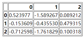
Of course read_ The HTML () method also supports reading HTML tables. Let's first generate a table like this through to_html() method
df = pd.DataFrame(np.random.randn(3, 3))
df.to_html("test_1.html")
Of course, this HTML form looks like this
Then we read_ The HTML method reads the file,
dfs = pd.read_html("test_1.html")
dfs[0]
read_csv() method and to_csv() method
read_csv() method
read_csv() method is one of the most commonly used methods for pandas to read data. The parameters we often use are
- filepath_or_buffer: the path of data input, which can be in the form of file path, for example
pd.read_csv('data.csv')
output
   num1  num2  num3  num4
0     1     2     3     4
1     6    12     7     9
2    11    13    15    18
3    12    10    16    18
It can also be a URL, if accessing the URL will return a file
pd.read_csv("http://...../..../data.csv")
- sep: the separator specified when reading csv files. The default is comma. Note that the separator of csv files should be consistent with the separator specified when reading csv files
Suppose that in our dataset, the separator in the csv file is changed from comma to "\ t", and the sep parameter needs to be set accordingly
pd.read_csv('data.csv', sep='\t')
- index_col: after reading the file, we can specify a column as the index of the DataFrame
pd.read_csv('data.csv', index_col="num1")
output
      num2  num3  num4
num1
1        2     3     4
6       12     7     9
11      13    15    18
12      10    16    18
In addition to specifying a single column, we can also specify multiple columns, such as
df = pd.read_csv("data.csv", index_col=["num1", "num2"])
output
           num3  num4
num1 num2
1    2        3     4
6    12       7     9
11   13      15    18
12   10      16    18
- usecols: if there are many columns in the dataset, and we don't want all the columns, but only the specified columns, we can use this parameter
pd.read_csv('data.csv', usecols=["Column name 1", "Column name 2", ....])
output
   num1  num2
0     1     2
1     6    12
2    11    13
3    12    10
In addition to specifying the column name, you can also select the desired column by index. The example code is as follows
df = pd.read_csv("data.csv", usecols = [0, 1, 2])
output
   num1  num2  num3
0     1     2     3
1     6    12     7
2    11    13    15
3    12    10    16
Another interesting thing about usecols parameters is that it can receive a function and pass the column name as a parameter to the function. If the condition is satisfied, the column will be selected, otherwise the column will not be selected.
# Select a column whose length is greater than 4
pd.read_csv('girl.csv', usecols=lambda x: len(x) > 4)
- Prefix: when the imported data does not have a header, it can be used to prefix the column name
df = pd.read_csv("data.csv", header = None)
output
      0     1     2     3
0  num1  num2  num3  num4
1     1     2     3     4
2     6    12     7     9
3    11    13    15    18
4    12    10    16    18
If we set the header to None, pandas will automatically generate headers 0, 1, 2, 3, Then we set the prefix parameter to prefix the header
df = pd.read_csv("data.csv", prefix="test_", header = None)
output
  test_0 test_1 test_2 test_3
0   num1   num2   num3   num4
1      1      2      3      4
2      6     12      7      9
3     11     13     15     18
4     12     10     16     18
- Skirows: which rows are filtered out, and the index of the rows filled in the parameters
The code is as follows:
df = pd.read_csv("data.csv", skiprows=[0, 1])
output
    6  12   7   9
0  11  13  15  18
1  12  10  16  18
The above code filters out the data of the first two lines and directly outputs the data of the third and fourth lines. Of course, we can also see that the data of the second line is regarded as the header
- nrows: this parameter sets the number of file lines read in at one time. It is very useful for reading large files. For example, a PC with 16G memory cannot accommodate hundreds of G large files
The code is as follows:
df = pd.read_csv("data.csv", nrows=2)
output
   num1  num2  num3  num4
0     1     2     3     4
1     6    12     7     9
to_csv() method
This method is mainly used to write DataFrame into csv file. The example code is as follows
df.to_csv("file name.csv", index = False)
We can also output to the format of zip file. The code is as follows
df = pd.read_csv("data.csv")
compression_opts = dict(method='zip',
                        archive_name='output.csv')
df.to_csv('output.zip', index=False,
          compression=compression_opts)
read_excel() method and to_excel() method
read_excel() method
If our data is stored in excel, we can use read_excel() method, and the parameters in this method are the same as the read mentioned above_ CSV () methods are not much different. We won't go into too much detail here. Let's look at the code directly
df = pd.read_excel("test.xlsx")
- dtype: this parameter can set the data type of a specified column
df = pd.read_excel("test.xlsx", dtype={'Name': str, 'Value': float})
output
    Name  Value
0  name1    1.0
1  name2    2.0
2  name3    3.0
3  name4    4.0
- sheet_name: set which sheet in excel to read
df = pd.read_excel("test.xlsx", sheet_name="Sheet3")
output
    Name  Value
0  name1     10
1  name2     10
2  name3     20
3  name4     30
Of course, if we want to read the data in multiple sheets at one time, the last returned data is returned in the form of dict
df = pd.read_excel("test.xlsx", sheet_name=["Sheet1", "Sheet3"])
output
{'Sheet1':     Name  Value
0  name1      1
1  name2      2
2  name3      3
3  name4      4, 'Sheet3':     Name  Value
0  name1     10
1  name2     10
2  name3     20
3  name4     30}
For example, we only want the data of Sheet1, so we can do this
df1.get("Sheet1")
output
    Name  Value
0  name1      1
1  name2      2
2  name3      3
3  name4      4
to_excel() method
In addition to writing DataFrame objects into Excel tables, the ExcelWriter() method also has similar functions. The code is as follows
df1 = pd.DataFrame([['A', 'B'], ['C', 'D']],
                   index=['Row 1', 'Row 2'],
                   columns=['Col 1', 'Col 2'])
df1.to_excel("output.xlsx")
Of course, we can also specify the name of the Sheet
df1.to_excel("output.xlsx", sheet_name='Sheet_Name_1_1_1')
Sometimes we need to output multiple DataFrame datasets to different sheets in one Excel
df2 = df1.copy()
with pd.ExcelWriter('output.xlsx') as writer:
    df1.to_excel(writer, sheet_name='Sheet_name_1_1_1')
    df2.to_excel(writer, sheet_name='Sheet_name_2_2_2')
We can also add another Sheet based on the existing Sheet
df3 = df1.copy()
with pd.ExcelWriter('output.xlsx', mode="a", engine="openpyxl") as writer:
    df3.to_excel(writer, sheet_name='Sheet_name_3_3_3')
We can generate it to Excel file and compress it
with zipfile.ZipFile("output_excel.zip", "w") as zf:
    with zf.open("output_excel.xlsx", "w") as buffer:
        with pd.ExcelWriter(buffer) as writer:
            df1.to_excel(writer)
Data in date format or date time format can also be processed accordingly
from datetime import date, datetime
df = pd.DataFrame(
    [
        [date(2019, 1, 10), date(2021, 11, 24)],
        [datetime(2019, 1, 10, 23, 33, 4), datetime(2021, 10, 20, 13, 5, 13)],
    ],
    index=["Date", "Datetime"],
    columns=["X", "Y"],
)
with pd.ExcelWriter(
    "output_excel_date.xlsx",
    date_format="YYYY-MM-DD",
    datetime_format="YYYY-MM-DD HH:MM:SS"
) as writer:
    df.to_excel(writer)
read_table() method
For txt files, you can use read_csv() method, or read_table() method, where the parameters and read_ The parameters in CSV () are roughly the same, so I won't go into too much detail here
df = pd.read_table("test.txt", names = ["col1", "col2"], sep=' ')
output
   col1  col2
0     1     2
1     3     4
2     5     6
3     7     8
4     9    10
5    11    12
The data in the txt file we want to read is separated by spaces, so we need to set the sep parameter to spaces
read_pickle() method and to_pickle() method
The Pickle module in Python implements the binary sequence and deserialization of a python object structure. The serialization process is to convert the text information into a binary data stream and save the data type at the same time. For example, in the process of data processing, if something suddenly needs to leave, you can directly serialize the data to the local. At this time, the type of data in processing is the same as that saved locally. After deserialization, it is also the data type, rather than processing from scratch
to_pickle() method
We first generate a pickle file from the DataFrame dataset to permanently store the data. The code is as follows
df1.to_pickle("test.pkl")
read_pickle() method
The code is as follows
df2 = pd.read_pickle("test.pkl")
read_xml() method and to_xml() method
XML refers to extensible markup language. Like JSON, it is also used to store and transfer data. It can also be used as a configuration file
Differences between XML and HTML
XML and HTML are designed for different purposes
- XML is designed to transmit and store data, focusing on the content of the data
- HTML is designed to display data, focusing on the appearance of the data
- XML will not replace HTML, but is a supplement to HTML
The best understanding of XML is an information transmission tool independent of software and hardware. Let's go through to first_ XML () method to generate XML data
df = pd.DataFrame({'shape': ['square', 'circle', 'triangle'],
                   'degrees': [360, 360, 180],
                   'sides': [4, np.nan, 3]})
df.to_xml("test.xml")
We use read in pandas_ XML () method to read data
df = pd.read_xml("test.xml")
output
      shape  degrees  sides
0    square      360    4.0
1    circle      360    NaN
2  triangle      180    3.0
read_clipboard() method
Sometimes data acquisition is inconvenient. We can copy it through read in Pandas_ The clipboard () method is used to read the copied data. For example, we select a part of the data, then copy it, and run the following code
df_1 = pd.read_clipboard()
output
   num1  num2  num3  num4
0     1     2     3     4
1     6    12     7     9
2    11    13    15    18
3    12    10    16    18
to_clipboard() method
If there is copy, there will be paste. We can output the DataFrame dataset to the clipboard and paste it into, for example, Excel table
df.to_clipboard()