PNAS

2018-ECCV-Progressive Neural Architecture Search

• Johns Hopkins University & Google AI & Stanford
• GitHub: 300+ stars
• Citation: 504

Motivation

current techniques usually fall into one of two categories: evolutionary algorithms(EA) or reinforcement learning(RL).

Although both EA and RL methods have been able to learn network structures that outperform manually designed architectures, they require significant computational resources.

The two current nas methods, EA and RL, have computational costs

Contribution

we describe a method that requiring 5 times fewer model evaluations during the architecture search.

Only one-fifth of the models need to be evaluated.

We propose to use heuristic search to search the space of cell structures, starting with simple (shallow) models and progressing to complex ones, pruning out unpromising structures as we go.

Incremental search, starting from the shallow network, gradually searches for complex networks.

Since this process is expensive, we also learn a model or surrogate function(Substitution function) which can predict the performance of a structure without needing to training it.

An evaluation function (predictor) that approximates the quality of a model is presented to directly predict model performance rather than training candidate networks from scratch.

Several advantages:

First, the simple structures train faster, so we get some initial results to train the surrogate quickly.

Proxy networks are small and fast (at a negligible cost).

Second, we only ask the surrogate to predict the quality of structures that are slightly different (larger) from the ones it has seen

The predictor only needs to predict slightly different networks.

Third, we factorize(decompose) the search space into a product(product) of smaller search spaces, allowing us to potentially search models with many more blocks.

Decomposition a large search space into the product of a small search space.

we show that our approach is 5 times more efficient than the RL method of [41] in terms of number of models evaluated, and 8 times faster in terms of total compute.

The efficiency is five times higher than that of the RL method and the total computation is eight times faster.

Method

Search Space

we first learn a cell structure, and then stack this cell a desired number of times, in order to create the final CNN.

Learn the cell structure first, then stack the cells to the target number of layers.

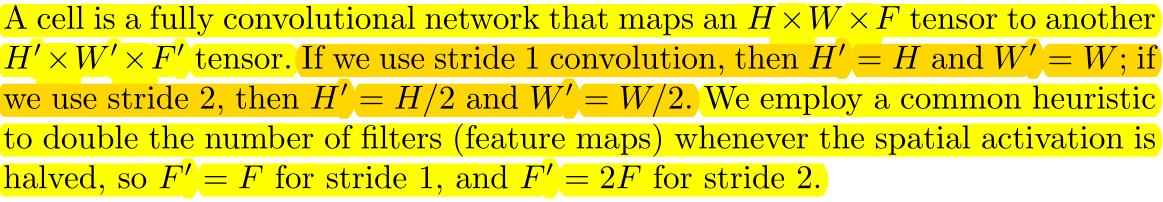
A cell receives a tensor of HxWxF, outputs a tensor of HxWxF if the cell's stride=1, and outputs a tensor of H/2 x W/2 x 2F if the cell's stride=2.

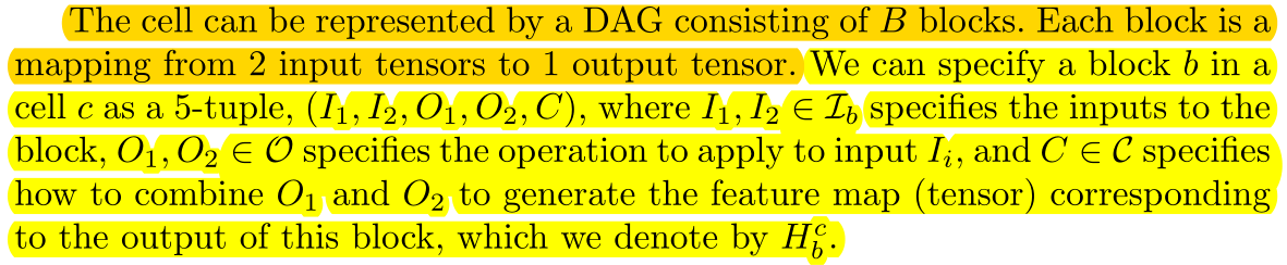
A cell consists of B blocks, with 2 input s and 1 output per block, and each block can be represented by a five-tuple \(left(I_{1}, I_{2}, O_{1}, O_{2}, C\right)\, the output of the CTH cell is represented as \(H^c\), and the output of the BTH block of the CTH cell is represented as \(H^c_b\).

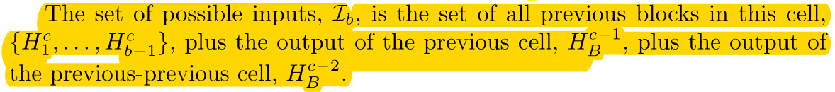
Each block's input is a collection of the output of all blocks before {this block} and {the output of the last cell, the output of the last cell} in the current cell.

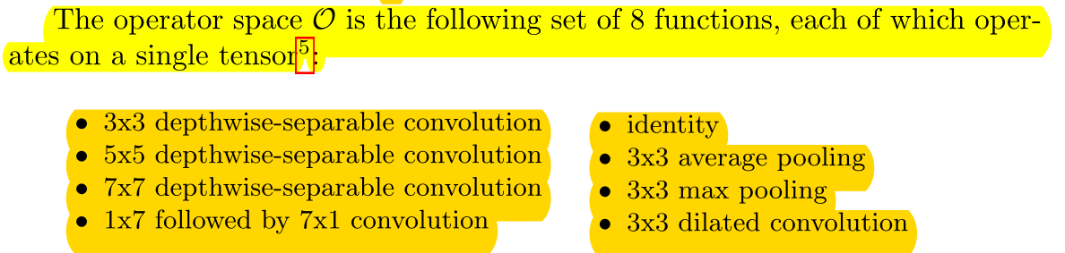
Operator has eight operations in its selection space.

we stack a predefined number of copies of the basic cell (with the same structure, but untied weights Do not inherit weights ), using either stride 1 or stride 2, as shown in Figure 1 (right).

After finding the best cell structure, stack the predefined number of layers to form the full network on the right, without inheriting the weights (retraining).

The number of stride-1 cells between stride-2 cells is then adjusted accordingly with up to N number of repeats.

The number of Normal cell s (stride=1) depends on N (superparameter).

we only use one cell type (we do not distinguish between Normal and Reduction cells, but instead emulate a Reduction cell by using a Normal cell with stride 2),

We do not distinguish between normal cell and Reduction cell, only set the stride of Normal cell to 2 as Reduction cell.

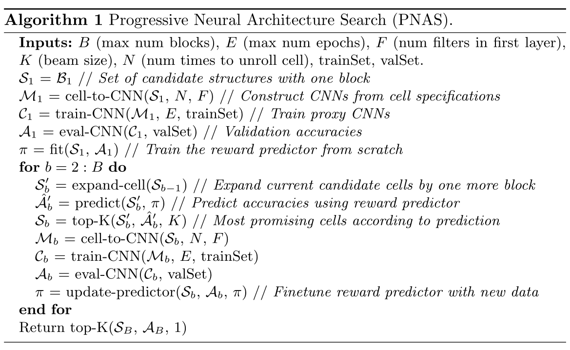
Progressive Neural Architecture Search

Many previous approaches directly search in the space of full cells, or worse, full CNNs.

The previous approach searched directly for the entire cell structure, or worse, the entire cnn.

While this is a more direct approach, we argue that it is difficult to directly navigate in an exponentially large search space, especially at the beginning where there is no knowledge of what makes a good model.

Although this approach is straightforward, the search space is too large and at first we don't have any prior knowledge to guide us in which direction to search in the vast search space.

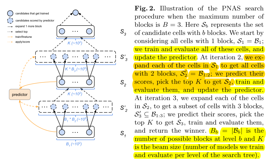
Search starts with one block per cell.Train all possible\(B_1\), with \(B_1\) Train the predictor, and then \(B_1\) Expand to \(B_2\).

Train all possible\(B_2\) is too expensive, so we use a predictor to evaluate all \(B_2\)-cell performance and select the best K\(B_2\- cell, repeat the process (with K selected\(B_2\)-cell training predictor, K\(B_will be selected2\) -cell expanded to \(B_3\) and select the best K with the predictor.

Performance Prediction with Surrogate Model

Requirement of Predictor:

• Handle variable-sized inputs
• Correlated with true performance
• Sample efficiency (simple and efficient)
• The requirement that the predictor be able to handle variable-sized strings immediately suggests the use of an RNN.

Two Predictor method

RNN and MLP (Multilayer Sensor)

However, since the sample size is very small, we fit an ensemble of 5 predictors, We observed empirically that this reduced the variance of the predictions.

Because the sample is simple, integrating five predictors (RNN-ensemble, MLP-ensemble) can reduce variance.

Experiments

Performance of the Surrogate Predictors

we train the predictor on the observed performance of cells with up to b blocks, but we apply it to cells with b+1 blocks.

Train on {B=b} and predict on the set of {B=b+1}.

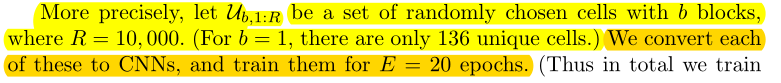
Randomly select 10k of all {B=b} cell collections as datasets\(U_{b, 1:R}\), training 20 epochs.

randomly select K = 256 models (each of size b) from \(U_{b,1 :R}\)to generate a training set \(S_{b,t,1:K}\);

256 training sets S were randomly selected from dataset U for each round.

A total of 20*256=5120 data points will be trained.

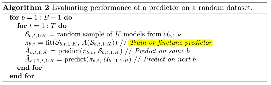
We now use this random dataset to evaluate the performance of the predictors using the pseudocode(Pseudocode) in Algorithm 2, where A(H) returns the true validation set accuracies of the models in some set H.

A(H) returns the true accuracy of the cell's set H after training.

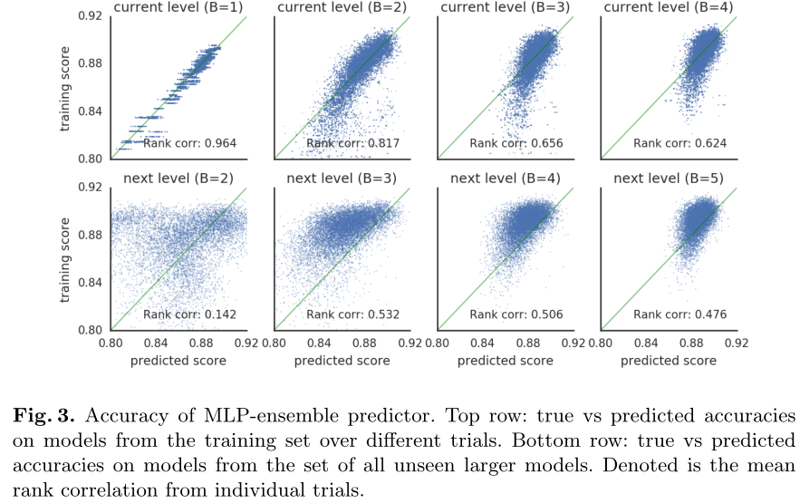
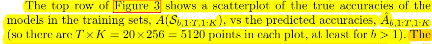
When B=b, the training set is a subset of all {B=b} cells. The first behavior is the correlation between predicted and real results on the training set (256*20=5120) of all {B=b} cells.
The second behavior is the correlation between predicted and true results on all {B=b+1} cell datasets (10k).

We see that the predictor performs well on models from the training set, but not so well when predicting larger models. However, performance does increase as the predictor is trained on more (and larger) cells.

The predictor performs well on the training set {B=b}, but does not perform well on the larger dataset {B=b+1}, but gets better as B increases.

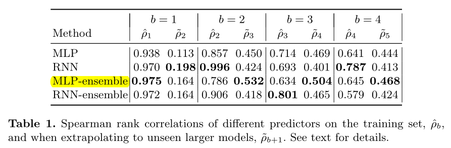
We see that for predicting the training set, the RNN does better than the MLP, but for predicting the performance on unseen larger models (which is the setting we care about in practice), the MLP seems to do slightly better.

The predictor of the RNN method performs better on the training set {B=b} and MLP performs better on the larger dataset {B=b+1} (we are concerned about)

Conclusion

The main contribution of this work is to show how we can accelerate the search for good CNN structures by using progressive search through the space of increasingly complex graphs

Accelerate NAS using progressive (cell-depth increasing) searches

combined with a learned prediction function to efficiently identify the most promising models to explore.

Use a learnable predictor to identify the potential optimal network.(A P-network is introduced to search for the optimal structure of the target network.eg. Use the C network to search for the best structure of the B network, and the B network is to search for the best structure of the A network, dolls)

The resulting models achieve the same level of performance as previous work but with a fraction of the computational cost.

SOTA achieved at a small price

Appendix