Write in front
This article will share the scheme of a recent game, which is a problem about time series. Although it did not reach the finals, many points are still worth learning. I hope it can help you, and welcome to have more discussions with me.
Here will also start from the code to share my problem-solving ideas.
text
1. Data description
The competition title gives the historical sales data, including the sales of 60 models in 22 provinces from January 2016 to December 2017. The participating teams need to predict the sales of these 60 models in 22 provinces in the next four months (January 2018 to April 2018); the participating teams need to divide the training set data for modeling.
Data files include:
[training set] historical sales data: train_sales_data_v1.csv
[training set] vehicle search data: train_search_data_v1.csv
[training set] vehicle vertical media news review data and vehicle model review data: train_user_reply_data_v1.csv
[evaluation set] sales forecast of various models and provinces from January to April 2018: evaluation_public.csv
There is not much difference between the preliminary and semi-finals, mainly due to the increase of models.
2. Evaluation indicators
In my opinion, the understanding of evaluation indicators can also help score.
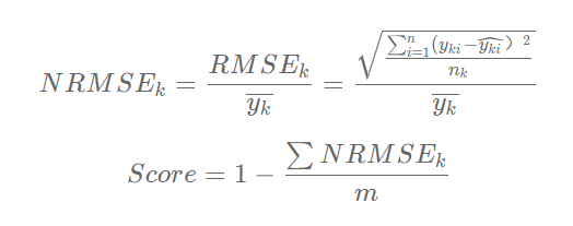
The average value of NRMSE (normalized root mean square error) is used as the evaluation index for online scoring in the preliminary and semi-final stages. First, the NRMSE of each vehicle model in each market segment (province) is calculated separately, and then the average value of all NRMSE is calculated. The calculation method is as follows:
Among them,

Model No

True values of samples,

For the first
Predicted values of samples,

Is the number of predicted samples of model k (n=4),

Is the average of the true values,

Is the number of models to be predicted.

As the final evaluation index, the value is between 0-1. The closer it is to 1, the more accurate the model is.
It's not difficult to understand that we need to score by model in different provinces, and then integrate them to get the final score.
The key is that such an evaluation index has a feature that the model with small sales will have a greater impact on the score. According to this feature, we can consider adding sample weight and the final fusion method.
The weight calculation method is given below. Of course, it is also constructed in an empirical way. There can be more optimizations.
# Sample weight information
data['n_salesVolume'] = np.log(data['salesVolume']+1)
df_wei = data.groupby(['province','model'])['n_salesVolume'].agg({'mean'}).reset_index().sort_values('mean')
df_wei.columns = ['province','model','wei']
df_wei['wei'] = 10 - df_wei['wei'].values
data = data.merge(df_wei, on=['province','model'], how='left')
Just add the weight information during the model training. There is a thousandth improvement in the preliminary competition, and there is no specific test in the second round.
dtrain = lgb.Dataset(df[all_idx][features], label=df[all_idx]['n_label'], weight=df[all_idx]['wei'].values)
The code of evaluation index is given below:
def score(data, pred='pred_label', label='label', group='model'):
    data['pred_label'] = data['pred_label'].apply(lambda x: 0 if x < 0 else x).round().astype(int)
    data_agg = data.groupby('model').agg({
        pred:  list,
        label: [list, 'mean']
    }).reset_index()
    data_agg.columns = ['_'.join(col).strip() for col in data_agg.columns]
    nrmse_score = []
    for raw in data_agg[['{0}_list'.format(pred), '{0}_list'.format(label), '{0}_mean'.format(label)]].values:
        nrmse_score.append(
            mse(raw[0], raw[1]) ** 0.5 / raw[2]
        )
    print(1 - np.mean(nrmse_score))
    return 1 - np.mean(nrmse_score)
3. Characteristic Engineering
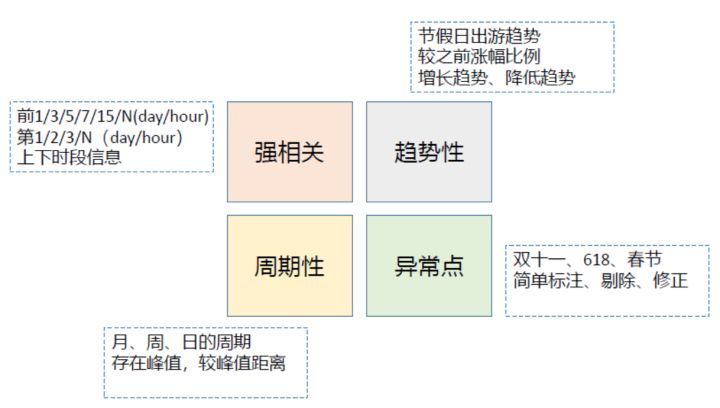
The scheme mainly constructs the traditional timing features, which are often extended from these aspects, or better describe these features. When faced with such problems, it must be right to consider these four points. In this competition, I have done little on abnormal aspects, and I have not found an effective way. However, I always firmly believe that I can't give a good score in terms of abnormal points.
The competition predicts the monthly car sales of models in provinces. We can extract features from different dimensions, either from the micro or macro point of view. I mainly consider the structure from two points, and also construct the relevant characteristics of popularity
1. province/Model/Month: car sales, popularity
2. Model/Month: car sales
How to select the specific interval and statistical method? Here is my plan
def getStatFeature(df_, month, flag=None):

    df = df_.copy()

    stat_feat = []

    # Determine starting position
    if (month == 26) & (flag):
        n = 1
    elif (month == 27) & (flag):
        n = 2
    elif (month == 28) & (flag):
        n = 3
    else:
        n = 0
    print('Starting position for statistics:',n,' month:',month)

    ######################
    # province/Model/Month granularity #
    #####################
    df['adcode_model'] = df['adcode'] + df['model']
    df['adcode_model_mt'] = df['adcode_model'] * 100 + df['mt']
    for col in tqdm(['label']):

        # translation
        start, end = 1+n, 9
        df, add_feat = get_shift_feature(df, start, end, col, 'adcode_model_mt')
        stat_feat = stat_feat + add_feat

        # adjacent
        start, end = 1+n, 8
        df, add_feat = get_adjoin_feature(df, start, end, col, 'adcode_model_mt', space=1)
        stat_feat = stat_feat + add_feat
        start, end = 1+n, 7
        df, add_feat = get_adjoin_feature(df, start, end, col, 'adcode_model_mt', space=2)
        stat_feat = stat_feat + add_feat
        start, end = 1+n, 6
        df, add_feat = get_adjoin_feature(df, start, end, col, 'adcode_model_mt', space=3)
        stat_feat = stat_feat + add_feat

        # continuity
        start, end = 1+n, 3+n
        df, add_feat = get_series_feature(df, start, end, col, 'adcode_model_mt', ['sum','mean','min','max','std','ptp'])
        stat_feat = stat_feat + add_feat
        start, end = 1+n, 5+n
        df, add_feat = get_series_feature(df, start, end, col, 'adcode_model_mt', ['sum','mean','min','max','std','ptp'])
        stat_feat = stat_feat + add_feat
        start, end = 1+n, 7+n
        df, add_feat = get_series_feature(df, start, end, col, 'adcode_model_mt', ['sum','mean','min','max','std','ptp'])
        stat_feat = stat_feat + add_feat

    for col in tqdm(['popularity']):

        # translation
        start, end = 4, 9
        df, add_feat = get_shift_feature(df, start, end, col, 'adcode_model_mt')
        stat_feat = stat_feat + add_feat

        # adjacent
        start, end = 4, 8
        df, add_feat = get_adjoin_feature(df, start, end, col, 'adcode_model_mt', space=1)
        stat_feat = stat_feat + add_feat
        start, end = 4, 7
        df, add_feat = get_adjoin_feature(df, start, end, col, 'adcode_model_mt', space=2)
        stat_feat = stat_feat + add_feat
        start, end = 4, 6
        df, add_feat = get_adjoin_feature(df, start, end, col, 'adcode_model_mt', space=3)
        stat_feat = stat_feat + add_feat

        # continuity
        start, end = 4, 7
        df, add_feat = get_series_feature(df, start, end, col, 'adcode_model_mt', ['sum','mean','min','max','std','ptp'])
        stat_feat = stat_feat + add_feat
        start, end = 4, 9
        df, add_feat = get_series_feature(df, start, end, col, 'adcode_model_mt', ['sum','mean','min','max','std','ptp'])
        stat_feat = stat_feat + add_feat

    ##################
    # Model/Month granularity #
    ##################
    df['model_mt'] = df['model'] * 100 + df['mt']
    for col in tqdm(['label']):
        colname = 'model_mt_{}'.format(col)
        tmp = df.groupby(['model_mt'])[col].agg({'mean'}).reset_index()
        tmp.columns = ['model_mt',colname]
        df = df.merge(tmp, on=['model_mt'], how='left')
        # translation
        start, end = 1+n, 9
        df, add_feat = get_shift_feature(df, start, end, colname, 'adcode_model_mt')
        stat_feat = stat_feat + add_feat

        # adjacent
        start, end = 1+n, 8
        df, add_feat = get_adjoin_feature(df, start, end, colname, 'model_mt', space=1)
        stat_feat = stat_feat + add_feat
        start, end = 1+n, 7
        df, add_feat = get_adjoin_feature(df, start, end, colname, 'model_mt', space=2)
        stat_feat = stat_feat + add_feat
        start, end = 1+n, 6
        df, add_feat = get_adjoin_feature(df, start, end, colname, 'model_mt', space=3)
        stat_feat = stat_feat + add_feat

        # continuity
        start, end = 1+n, 3+n
        df, add_feat = get_series_feature(df, start, end, colname, 'model_mt', ['sum','mean'])
        stat_feat = stat_feat + add_feat
        start, end = 1+n, 5+n
        df, add_feat = get_series_feature(df, start, end, colname, 'model_mt', ['sum','mean'])
        stat_feat = stat_feat + add_feat
        start, end = 1+n, 7+n
        df, add_feat = get_series_feature(df, start, end, colname, 'model_mt', ['sum','mean'])
        stat_feat = stat_feat + add_feat

    return df,stat_feat
There are three functions involved:
def get_shift_feature(df_, start, end, col, group):
    '''
    Historical translation feature
    col  : label,popularity
    group: adcode_model_mt, model_mt
    '''
    df = df_.copy()
    add_feat = []
    for i in range(start, end+1):
        add_feat.append('shift_{}_{}_{}'.format(col,group,i))
        df['{}_{}'.format(col,i)] = df[group] + i
        df_last = df[~df[col].isnull()].set_index('{}_{}'.format(col,i))
        df['shift_{}_{}_{}'.format(col,group,i)] = df[group].map(df_last[col])
        del df['{}_{}'.format(col,i)]

    return df, add_feat

def get_adjoin_feature(df_, start, end, col, group, space):
    '''
    adjacent N Beginning and end statistics of the month
    space: interval
    Notes: shift Unified as adcode_model_mt
    '''
    df = df_.copy()
    add_feat = []
    for i in range(start, end+1):
        add_feat.append('adjoin_{}_{}_{}_{}_{}_sum'.format(col,group,i,i+space,space)) # Sum
        add_feat.append('adjoin_{}_{}_{}_{}_{}_mean'.format(col,group,i,i+space,space)) # mean value
        add_feat.append('adjoin_{}_{}_{}_{}_{}_diff'.format(col,group,i,i+space,space)) # Head tail difference
        add_feat.append('adjoin_{}_{}_{}_{}_{}_ratio'.format(col,group,i,i+space,space)) # Head to tail ratio
        df['adjoin_{}_{}_{}_{}_{}_sum'.format(col,group,i,i+space,space)] = 0
        for j in range(0, space+1):
            df['adjoin_{}_{}_{}_{}_{}_sum'.format(col,group,i,i+space,space)]   = df['adjoin_{}_{}_{}_{}_{}_sum'.format(col,group,i,i+space,space)] +\
                                                                                  df['shift_{}_{}_{}'.format(col,'adcode_model_mt',i+j)]
        df['adjoin_{}_{}_{}_{}_{}_mean'.format(col,group,i,i+space,space)]  = df['adjoin_{}_{}_{}_{}_{}_sum'.format(col,group,i,i+space,space)].values/(space+1)
        df['adjoin_{}_{}_{}_{}_{}_diff'.format(col,group,i,i+space,space)]  = df['shift_{}_{}_{}'.format(col,'adcode_model_mt',i)].values -\
                                                                              df['shift_{}_{}_{}'.format(col,'adcode_model_mt',i+space)]
        df['adjoin_{}_{}_{}_{}_{}_ratio'.format(col,group,i,i+space,space)] = df['shift_{}_{}_{}'.format(col,'adcode_model_mt',i)].values /\
                                                                              df['shift_{}_{}_{}'.format(col,'adcode_model_mt',i+space)]
    return df, add_feat

def get_series_feature(df_, start, end, col, group, types):
    '''
    continuity N Monthly statistics
    Notes: shift Unified as adcode_model_mt
    '''
    df = df_.copy()
    add_feat = []
    li = []
    df['series_{}_{}_{}_{}_sum'.format(col,group,start,end)] = 0
    for i in range(start,end+1):
        li.append('shift_{}_{}_{}'.format(col,'adcode_model_mt',i))
    df['series_{}_{}_{}_{}_sum'.format( col,group,start,end)] = df[li].apply(get_sum, axis=1)
    df['series_{}_{}_{}_{}_mean'.format(col,group,start,end)] = df[li].apply(get_mean, axis=1)
    df['series_{}_{}_{}_{}_min'.format( col,group,start,end)] = df[li].apply(get_min, axis=1)
    df['series_{}_{}_{}_{}_max'.format( col,group,start,end)] = df[li].apply(get_max, axis=1)
    df['series_{}_{}_{}_{}_std'.format( col,group,start,end)] = df[li].apply(get_std, axis=1)
    df['series_{}_{}_{}_{}_ptp'.format( col,group,start,end)] = df[li].apply(get_ptp, axis=1)
    for typ in types:
        add_feat.append('series_{}_{}_{}_{}_{}'.format(col,group,start,end,typ))

    return df, add_feat
See here, my features are basically finished. There is no complex structure, and they are relatively basic.
There is still a part of the above code that hasn't been explained clearly
    # Determine starting position
    if (month == 26) & (flag):
        n = 1
    elif (month == 27) & (flag):
        n = 2
    elif (month == 28) & (flag):
        n = 3
    else:
        n = 0
This part is mainly used to determine the starting position of the extracted features, mainly in the selection of modeling methods.
4. Modeling strategy
The test set needs to predict the car sales in four months. There are still many modeling strategies available. The main personal scheme is to predict step by step. First, get the results in January, and then merge January into the training set to predict the results in February, then March and April.
In this way, errors may be accumulated, and all can also be extracted by jumping.
for month in [25,26,27,28]:

    m_type = 'xgb'
    flag = False # False: continuous extraction True: skip extraction
    st = 4 # Keep training set start position

    # Feature extraction
    data_df, stat_feat = get_stat_feature(data, month, flag)

    # Feature classification
    num_feat = ['regYear'] + stat_feat
    cate_feat = ['adcode','bodyType','model','regMonth']

    # Category feature processing
    if m_type == 'lgb':
        for i in cate_feat:
            data_df[i] = data_df[i].astype('category')
    elif m_type == 'xgb':
        lbl = LabelEncoder()
        for i in tqdm(cate_feat):
            data_df[i] = lbl.fit_transform(data_df[i].astype(str))

    # Final feature set
    features = num_feat + cate_feat
    print(len(features), len(set(features)))

    # model training
    sub, model = get_train_model(data_df, month, m_type, st)

    data.loc[(data.regMonth==(month-24))&(data.regYear==2018), 'salesVolume'] = sub['forecastVolum'].values
    data.loc[(data.regMonth==(month-24))&(data.regYear==2018), 'label'      ] = sub['forecastVolum'].values
Here m_type determines the selected model, flag determines whether to sample the spanning feature extraction, and st retains the starting position of the training set. Basically, the final scheme is only modified on these parameters and then fused.
5. Integration mode
There can also be many fusion methods, stacking and blending. Only blending is selected here, and the two weighting methods, arithmetic average and geometric average, are tried.
Arithmetic mean:

Geometric average:

Due to the scoring rules, the arithmetic average will make the fusion result too large, such as:
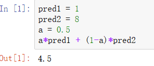
Obviously, it is not in line with the intuition of the evaluation index of this competition. The smaller the value, the greater the impact on the score, and the arithmetic average will lead to greater error. Therefore, selecting geometric average can bias the results to small values, as follows:
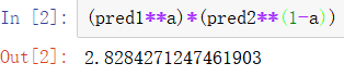
This operation is also the final score has nearly a thousand improvements. This method has also been used in previous competitions, which is very worthy of reference. The in the recent "National University new energy innovation competition" is still applicable.