Lightweight C + + neural network application library CreativeLus: 3. Complex function approximation. Case: multi input mixed approximation.

github resource address:[ Release-x86/x64]

Last article: Lightweight C + + neural network application library CreativeLus: 2. Classification problem. Case: space points are classified in plane 2.
Next article: Creative LUS: 4. CNN convolutional neural network. Case: (MNIST) handwritten digit recognition.

Case 3: complex function approximation

This chapter introduces the following main contents, which are very important:
1. Create the neural network of self defining structure;
2. Introduction of model self adjustment (not parameter adjustment);
3. Customize process monitoring and output.

Problem description of this example

In order to show the strong approximation ability of neural network, we will[ Case 1: approximation of simple sin function ]Through the complex multi input and multi output approximation problem, we can understand the operation mode of neural network.

The proposition is as follows: define the input vector X={x1,x2,x3,x4} of dimension 4, where xi is the random value of ∈ [- π, π], and get the output vector y of dimension 4 by mapping γ (X), that is, y = γ (X)={y1,y2,y3,y4}={sin(x4),cos(x3),min(0.1ex2,1),min(1/(1+e(- x1)),1)}, where yi ∈ [- 1,1]. From the random input of [− π, π] to the cross output of [− 1,1], a training set is formed. Construct appropriate neural network, find the mapping relationship γ through training, and verify the validity of the model through random input proposition as follows: E ^ {(- x_1)}), 1) \}, where yi\in\mathbb [-1,1]. From the random input of [- \ pi,\pi] to the cross output of [- 1,1], the training set is formed. Construct an appropriate neural network, find the mapping relationship \ Gamma through training, and verify the validity of the model through random input proposition as follows: define the input vector X={x1, x2, X3, X4} with dimension 4, where xi is the random value of ∈ [- π, π], and get the output vector y with dimension 4 through mapping Γ (X), that is, y = Γ (X)={y1, y2, y3, y4} = {sin(x4), cos(x3), min(0.1ex2 , 1),min(1/(1+e(− x1)), 1)}, where yi ∈ [− 1,1]. From the random input of [− π, π] to the cross output of [− 1,1], a training set is formed. Construct the appropriate neural network, find the mapping relation γ by training, and verify the validity of the model by random input

Map the true relationship of γ \ Gamma γ. The code snippet is as follows:

const Float rangA = -ConstPi * 1.0, rangB = ConstPi * 1.0;
Float x4 = 0, x1 = 0, x2 = 0, x3 = 0, y4 = 0, y1 = 0, y2 = 0, y3 = 0;
#define XData3 x1 = rand_f_a_b(rangA,rangB),x2 = rand_f_a_b(rangA,rangB),x3 = rand_f_a_b(rangA,rangB),x4 = rand_f_a_b(rangA,rangB)
#define YData3 y1 = sin(x4),y2 = cos(x3),y3 = min(exp(x2)*0.1,1),y4 = min((1.0/(1.0+exp(-x1))),1)

1. "Creativity decides everything", design your own neural network

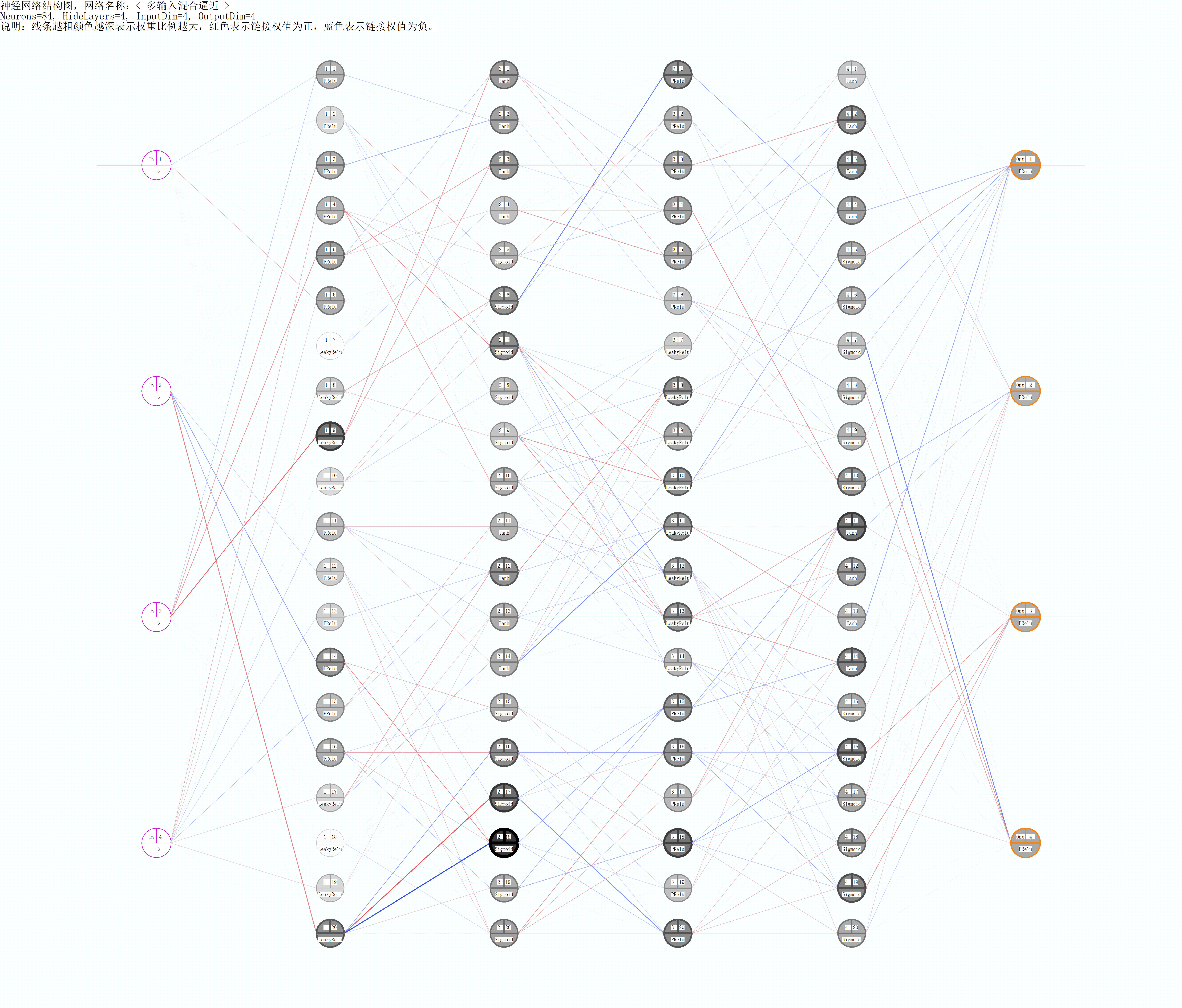
Let's not say much. Let's take a look first. In order to find the approximation mapping relationship for the problem in this case, we "designed" the network model (5-layer, 4-input, 4-output model structure) as shown in the figure below to solve the above problem.

It's obviously a little deliberate to deal with the approximation problem, which is just called design, and make the structure like this, but in order to demonstrate, we should try to make it more complex and beautiful. If you're tired of the monotonous, stereotyped model structure. Then it's time for you to show your skills, all of which will come from your creativity.

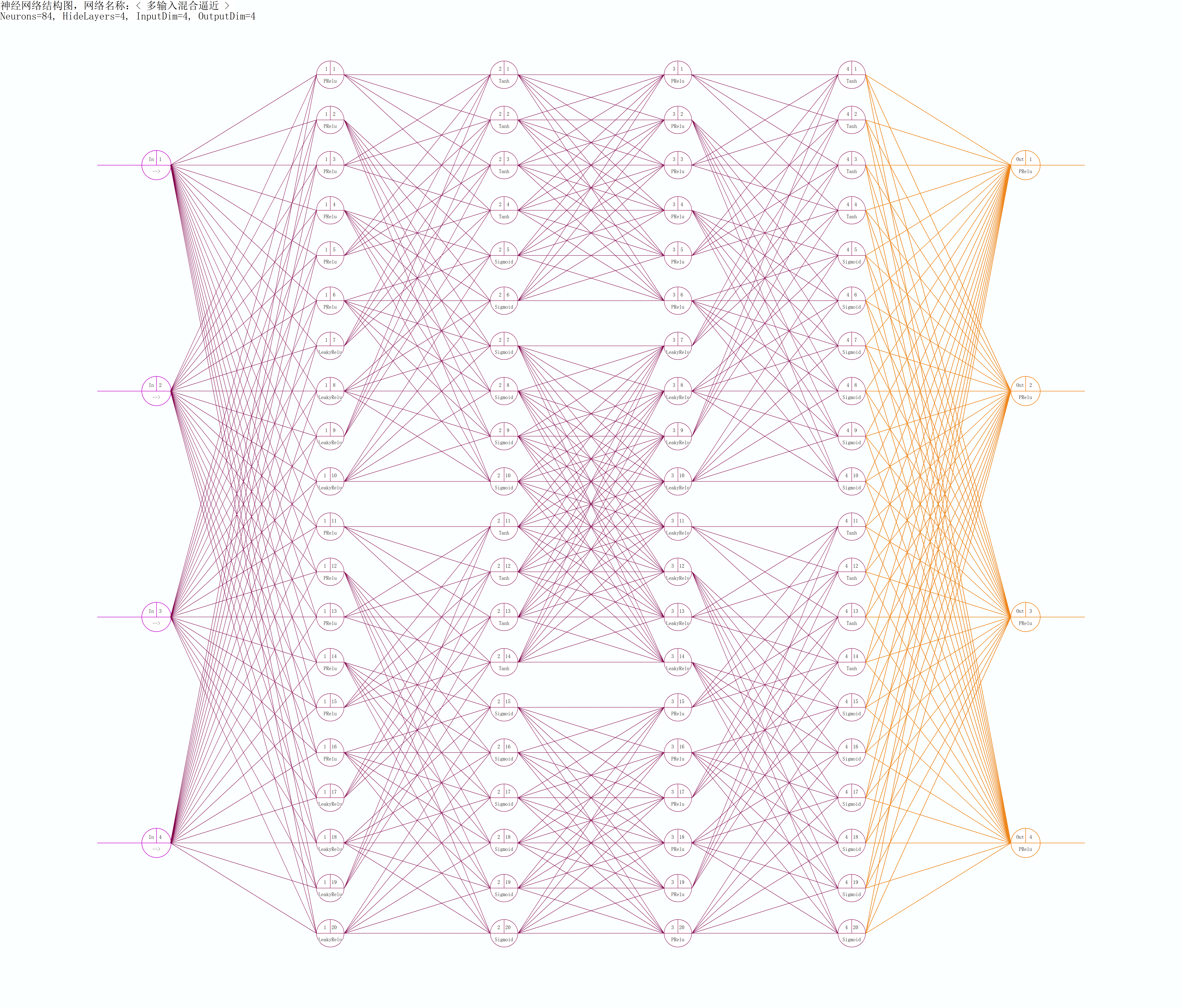
The picture is automatically generated by CL, which can be zoomed in and out with the left mouse button and CSCEC.
It can be observed that in this model, we use four different activation functions: Sigmoid, Tanh, PReLu, LeakyReLu (for the functions of the above four functions, please do not discuss them here). Secondly, each neuron is represented as a node, which links the previous layer (on the left), and is linked by the next layer (on the right), which transfers from left to right. The connection of neurons is not regular, but selective. CL is object-oriented modeling, each neuron is an independent individual, it knows what it is to do.

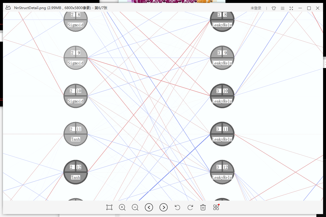
In the following figure, the network structure with weight rendering is shown:

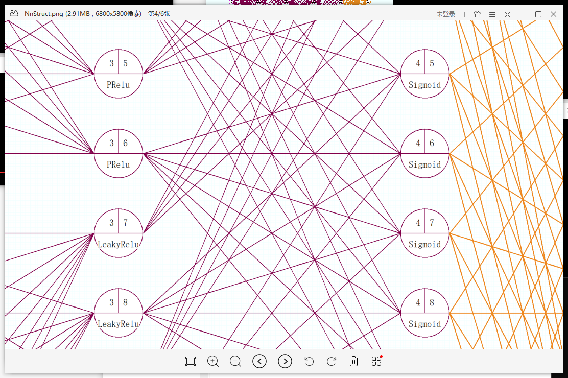
Local network structure with weight:

If you think it takes a lot of effort to make such a model, you are wrong. To complete such a work, you only need 5 lines of code. The construction code is as follows, with a large number of comments, which introduces the method of using BpnnStructDef to define the network structure. Class BpnnStructDef is the key medium for CL to build custom network. (for this case, see Appendix 1 of this chapter for the complete code)

        ///////////////////////////////////////////////////////////////////////////////
		// Custom network:
		// Concept description: CL is an object-oriented modeling of neurons. Each neuron should know what it is, what functions it has, who it links (similar to biological neuron dendrites), how to process the data transferred to the neuron core, how to activate the data after transmission and processing, etc.

		// The following is the assembly of BpnnStructDef structure through the displayed definition to complete the customization of network structure (this is also the necessary method to realize the customization of network structure, which is very important)
		// The smallest definition unit is a BSB structure: BSB, which describes the attributes of the same neuron (i.e. all attributes are identical) in this layer,
		// The BSB structure describes: the number of the same neurons in this group, the type of transfer function, which upper nodes are linked (which is very important), and the processing method of the incoming data of the upper linked nodes (such as: linear addition, Max, Min, and mean, which are used in CNN pooling operation of convolution network),
		// Weight and threshold initialization scheme, whether to use shared weight (used in convolution network CNN).
		BpnnStructDef mod = { 
			// Construct the first layer (which directly accepts all dimensions of input data):
			// Taking the first BSB as an example, it expresses that there are six identical neurons in this group, and the transfer function is PRelu. Because there is no link description defined for the upper layer, this group adopts the full connection for the upper layer (you can also specify the link if necessary);
			// There are 4 groups in this layer, and the number of neurons in each group is different. Therefore, the total number of neurons in this layer is the sum of the number of neurons in each group, that is, there are 6 + 4 + 6 + 4 = 20 neurons in the first layer, and this layer has been defined;			
			{BSB(6,TF_PRelu),BSB(4,TF_LeakyRelu,{}),BSB(6,TF_PRelu),BSB(4,TF_LeakyRelu,{})},
			
			// Construct the second layer: four groups (four BSB structures) in total. Take the first group (BSB) as an example: there are four neurons in this group, the transfer function is Tanh, and the number of neurons linked to the previous layer is {1,3,5,7,9}
			// Note that the upper link number is counted from 1, not 0, pay special attention; if the upper link number is not specified (similar to the case of the first layer), the method of full connection to the upper layer will be adopted.
			{BSB(4,TF_Tanh,{1,3,5,7,9}),BSB(6,TF_Sigmoid,{2,4,6,8,10}),BSB(4,TF_Tanh,{11,13,15,17,19}),BSB(6,TF_Sigmoid,{12,14,16,18,20})},
			
			// The third layer (customized according to requirements, the method is the same as above, only for demonstration here)
			{BSB(6,TF_PRelu,{1,2,3,4,5,6}),BSB(8,TF_LeakyRelu,{7,8,9,10,11,12,13,14}),BSB(6,TF_PRelu,{15,16,17,18,19,20})},
			
			// The fourth layer (customized according to the requirements, the method is the same as above, only for demonstration here)
			{BSB(4,TF_Tanh,{1,3,5,7,9}),BSB(6,TF_Sigmoid,{2,4,6,8,10}),BSB(4,TF_Tanh,{11,13,15,17,19}),BSB(6,TF_Sigmoid,{12,14,16,18,20})},
			
			// The last layer (output layer, which must be defined): because of our problems, the output dimension must be 4, so the total number of neurons constructed by the output layer must also be 4 (independent of the number of BSB, only related to the total number of neurons in this layer), and the upper layer also adopts full connection
			{BSB(4,TF_PRelu)},

		};// So far, we have completed a 4-output, 5-layer neural network structure definition. In the future, only the mod needs to be selected into bp, and the self defined network can be generated through buildNet.
		
		// Conclusion: many complex network structures can be realized by using simple BSB unit to construct the network, through free and flexible combination. Later, we will see similar: standard and non-standard convolution layer, softmax classifier, perception structure, residual network ResNet can be constructed.
		///////////////////////////////////////////////////////////////////////////////

2. "Correct when you know something wrong", model self-adjusting learning rate, repair calculation

In the code of this case, we accidentally set the learning rate too high.

Float learnRate = 100.1; // The learning rate is set to 100, please refer to Appendix 1: complete code
Float tagEr = 0.0001, movment = 0.8;
bp.setParam(learnRate, tagEr, movment);

Model training process gradient explosion. However, it doesn't matter. CL will automatically adjust the excessive learning rate to the appropriate initial size. Before adjustment, the following prompt window will pop up to ask for the user's opinions and choose whether to adjust or exit. If the user has been waiting after the prompt box appears, 10 seconds later, the system will automatically close the prompt and press No to continue.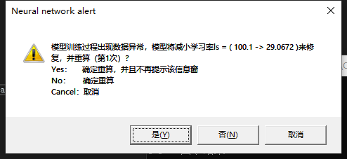

Note: if the data exception is still detected after multiple adjustments during model training (up to 15 checks), the adjustment and reset will not continue, but the data exception will be thrown.
In this example, the output adjustment process is output to the console through the monitor, and the effect is as follows:

[Waring]: Times= 1'st.The model automatically adjust learning rate ( 100.1 -> 29.0672 ) and retry!
[Waring]: Times= 2'st.The model automatically adjust learning rate ( 29.0672 -> 6.89407 ) and retry!
[Waring]: Times= 3'st.The model automatically adjust learning rate ( 6.89407 -> 1.01794 ) and retry!
[Waring]: Times= 4'st.The model automatically adjust learning rate ( 1.01794 -> 0.115428 ) and retry!
[Waring]: Times= 5'st.The model automatically adjust learning rate ( 0.115428 -> 0.0279845 ) and retry!

3. "Process information output", define your own process monitor

Case 1,Case 2 We used a built-in process monitor, which provides a callback function pointer to the process to be monitored. It mainly monitors the two time-consuming processes of buildNet construction network and train training network.

//code snippet
Bpnn::CallBackExample bk; //Bpnn::CallBackExample is a monitor that implements echo function
BPNN_CALLBACK_MAKE(vcb2, Bpnn::CallBackExample::print);//BPNN ﹣ callback ﹣ make is a macro that constructs a pointer to a monitoring callback function

bp.buildNet(vcb2, &bk); //Monitor incoming method, monitor construction process
bp.train(0, 0, 0, vcb2, &bk);//Monitor training process

There are many ways to quickly customize a monitor. For example, static, global, lambda expression, or class member function can be constructed. The class Bpnn::CallBackExample uses the class member function as the callback scheme to achieve the console output echo effect.
Here's a quick way to build a monitor with lambda expressions:

		// Mode 1: 
		// Define the static function pointer Bpnn::CbFunStatic pMonit, and quickly create a monitor through lambda
		Bpnn::CbFunStatic pMonit = [](Int c, Int max, PCStr inf) { 
			// c is the current information number id, max is the total information number, and inf is the information string;
			// When c < 0, a prompt message is passed in; when c and max are > = 0, a process message is passed in;
			if (c < 0) {
				cout << endl                      << "[Info ]" << inf;
			}
			else {
				if (c == 1) { cout << endl        << "[Start]" << inf; }
				else if (c == max) { cout << endl << "[Done ]" << inf; }
			}
		};
		
		bp.buildNet(pMonit);//Monitoring callback pointer in
		bp.train(0, 0, 0, pMonit);

Output effect: the part with brackets [] is the effect of monitor output information.

//Case 3: multi input hybrid approximation

[Start]Net is building hide layer.
[Done ]Net is building hide layer.
[Info ]Net construct completed. Neurons: 84, layers: 5.
[Start]Net is checking share link range.
[Done ]Net is checking share link range.
[Start]Net is training.
[Info ][Waring]: Times= 1'st.The model automatically adjust learning rate ( 100.1 -> 14.6937 ) and retry!
[Start]Net is checking share link range.
[Done ]Net is checking share link range.
[Start]Net is training.
[Info ][Waring]: Times= 2'st.The model automatically adjust learning rate ( 14.6937 -> 3.87114 ) and retry!
[Start]Net is checking share link range.
[Done ]Net is checking share link range.
[Start]Net is training.
[Info ][Waring]: Times= 3'st.The model automatically adjust learning rate ( 3.87114 -> 1.05257 ) and retry!
[Start]Net is checking share link range.
[Done ]Net is checking share link range.
[Start]Net is training.
[Info ][Waring]: Times= 4'st.The model automatically adjust learning rate ( 1.05257 -> 0.115818 ) and retry!
[Start]Net is checking share link range.
[Done ]Net is checking share link range.
[Start]Net is training.
[Info ][Waring]: Times= 5'st.The model automatically adjust learning rate ( 0.115818 -> 0.0183949 ) and retry!
[Start]Net is checking share link range.
[Done ]Net is checking share link range.
[Start]Net is training.
[Done ]Net is training.
[Info ]Net training epoch completed.
Epoch 1: Total time consumption:27.1134Seconds, this time:27.1134Second, CorrectRate = 55.07 %, Er = 6.78812e-05

[Start]Net is training.
[Done ]Net is training.
[Info ]Net training epoch completed.
Epoch 2: Total time consumption:42.0107Seconds, this time:14.8973Second, CorrectRate = 66.40 %, Er = 9.02233e-05

[Start]Net is training.
[Done ]Net is training.
[Info ]Net training epoch completed.
Epoch 3: Total time consumption:55.4777Seconds, this time:13.467Second, CorrectRate = 70.40 %, Er = 7.65581e-05

github resource address:[ Release-x86/x64]

Appendix:

Appendix 1: complete code

#include <stdio.h>
#include <string>
#include <vector>
#include <map>
#include "CreativeLus.h"

using namespace cl;

int main() {
	printf("\n\n//Case 3: multiple input mixed approximation \ n“);
	string pathTag = ("D:\\Documents\\Desktop\\example_02_multi_approach\\"); //Output directory

	const Float rangA = -ConstPi * 1.0, rangB = ConstPi * 1.0;
	Float x4 = 0, x1 = 0, x2 = 0, x3 = 0, y4 = 0, y1 = 0, y2 = 0, y3 = 0;
#define XData3 x1 = rand_f_a_b(rangA,rangB),x2 = rand_f_a_b(rangA,rangB),x3 = rand_f_a_b(rangA,rangB),x4 = rand_f_a_b(rangA,rangB)
#define YData3 y1 = sin(x4),y2 = cos(x3),y3 = min(exp(x2)*0.1,1),y4 = min((1.0/(1.0+exp(-x1))),1)
#define LDataIn3  x1,x2,x3,x4
#define LDataOut3 y1,y2,y3,y4

	Bpnn bp;
	Float learnRate = 100.1;
	Float tagEr = 0.0001, movment = 0.8;
	if (!bp.readBpnnFormFile((pathTag + "model1.txt").c_str())) {  //Read the model result file, if it exists, it will no longer be trained, direct prediction (only for demonstration here, not necessary)
		// Step 1: construct the dataset-------------------------------
		BpnnSamSets sams;
		BpnnSamSets tags;
		size_t nPtSi = 3000;
		for (size_t i = 0; i < nPtSi; i++) {
			XData3; YData3; sams.addSample({ LDataIn3 }, { LDataOut3 });
			XData3; YData3; tags.addSample({ LDataIn3 }, { LDataOut3 });
		}
		sams.writeToFile((pathTag + "sams.txt").c_str());
		tags.writeToFile((pathTag + "tags.txt").c_str());


		//Part two: network construction------------------------------

		///////////////////////////////////////////////////////////////////////////////
		// Custom network:
		// Concept description: CL is an object-oriented modeling of neurons. Each neuron should know what it is, what functions it has, who it links (similar to biological neuron dendrites), how to process the data transferred to the neuron core, how to activate the data after transmission and processing, etc.

		// The following is the assembly of BpnnStructDef structure through the displayed definition to complete the customization of network structure (this is also the necessary method to realize the customization of network structure, which is very important)
		// The smallest definition unit is a BSB structure: BSB describes the definition of the same neuron (i.e. all attributes are identical) in this layer,
		// BSB describes: the number of the same neurons in this group, the type of transfer function, which upper nodes are linked (which is very important), and the processing method of the incoming data of the upper linked nodes (such as linear addition, Max, Min, and mean, which are used in CNN pooling operation of convolution network),
		// Weight and threshold initialization scheme, whether to use shared weight (used in convolution network CNN).
		BpnnStructDef mod = { 
			// Construct the first layer (which directly accepts all dimensions of input data):
			// Taking the first BSB as an example, it expresses that there are six identical neurons in this group, and the transfer function is PRelu. Because there is no link description defined for the upper layer, this group adopts the full connection for the upper layer (you can also specify the link if necessary);
			// There are 4 groups in this layer, and the number of neurons in each group is different. Therefore, the total number of neurons in this layer is the sum of the number of neurons in each group, that is, there are 6 + 4 + 6 + 4 = 20 neurons in the first layer, and this layer has been defined;
			{BSB(6,TF_PRelu),BSB(4,TF_LeakyRelu,{}),BSB(6,TF_PRelu),BSB(4,TF_LeakyRelu,{})},

			// Construct the second layer: four groups (four BSB structures) in total. Take the first group (BSB) as an example: there are four neurons in this group, the transfer function is Tanh, and the number of neurons linked to the previous layer is {1,3,5,7,9}
			// Note that the upper link number is counted from 1, not 0, pay special attention; if the upper link number is not specified (similar to the case of the first layer), the method of full connection to the upper layer will be adopted.
			{BSB(4,TF_Tanh,{1,3,5,7,9}),BSB(6,TF_Sigmoid,{2,4,6,8,10}),BSB(4,TF_Tanh,{11,13,15,17,19}),BSB(6,TF_Sigmoid,{12,14,16,18,20})},
			// The third layer (customized according to requirements, the method is the same as above, only for demonstration here)
			{BSB(6,TF_PRelu,{1,2,3,4,5,6}),BSB(8,TF_LeakyRelu,{7,8,9,10,11,12,13,14}),BSB(6,TF_PRelu,{15,16,17,18,19,20})},
			// The fourth layer (customized according to the requirements, the method is the same as above, only for demonstration here)
			{BSB(4,TF_Tanh,{1,3,5,7,9}),BSB(6,TF_Sigmoid,{2,4,6,8,10}),BSB(4,TF_Tanh,{11,13,15,17,19}),BSB(6,TF_Sigmoid,{12,14,16,18,20})},
			// The last layer (output layer, which must be defined): because of our problems, the output dimension must be 4, so the total number of neurons constructed by the output layer must also be 4 (independent of the number of BSB, only related to the total number of neurons in this layer), and the upper layer also adopts full connection
			{BSB(4,TF_PRelu)},

		};// So far, we have completed a 4-output, 5-layer neural network structure definition. In the future, only the mod needs to be selected into bp, and the self defined network can be generated through buildNet.
		
		// Conclusion: many complex network structures can be realized by using simple BSB unit to construct the network, through free and flexible combination. Later, we will see similar: standard and non-standard convolution layer, softmax classifier, perception structure, residual network ResNet can be constructed.
		///////////////////////////////////////////////////////////////////////////////

		mod.writeToFile((pathTag + "NnStructDef.txt").c_str());//The structure definition can be output and saved as a text file. You can open and view the content by yourself		

		
		bp.setName("Multi input mixed approximation");
		bp.setSampSets(sams);
		bp.setCorrectRateEvaluationModel(0.985, &tags,tags.size() / 4,true);

		bp.setStructure(mod); //Note: select the structure definition object into the model before buildNet and set the model construction scheme (very important)
		//{{{
		bp.setLayer(3, 28); //Due to the use of BpnnStructDef to customize the network structure, the layer and node data set by this method will be invalid and ignored (only for demonstration here, no practical significance)
		bp.setTransFunc(TF_Sigmoid, TF_PRelu); //Due to the use of BpnnStructDef to customize the network structure, the transfer functions of each layer set in this method will be invalid and ignored (only for demonstration here, no practical significance)
		//}}}

		bp.setSampleBatchCounts(40, true);  //Set the number of samples in a batch and use random sampling
		bp.setParam(learnRate, tagEr, movment);   
		bp.setMultiThreadSupport(true);	   //Multi thread acceleration is adopted. (CPU requires a minimum of 4 cores)
		bp.setMaxTimes(sams.size() * 20);
		bp.openGraphFlag(true);
		Bpnn::CallBackExample bk;
		BPNN_CALLBACK_MAKE(vcb2, Bpnn::CallBackExample::print);//Construct monitoring callback function pointer
		bp.buildNet(vcb2, &bk);
		bp.exportGraphNetStruct((pathTag + "NnStruct.bmp").c_str());//After constructing the network, output the network structure to the bmp picture file


		CLTick tick, tick2, tick3; 
		bool rt = false; Int epoch = 0;
		while (!rt) {
			rt = bp.train(0, 0, 0, vcb2, &bk);
			printf(("Epoch %d: Total time consumption:%g Seconds, this time:%g Second, CorrectRate = %.2f %%, Er = %g \n\n"), ++epoch, tick.getSpendTime(), tick2.getSpendTime(true),
				bp.getSavedCorrectRate() * 100.0, bp.getEr());
			if (epoch == 1 || rt == true || tick3.getSpendTime() > 20.0) {
				bp.showGraphParam(0); //When all data is displayed for 0
				bp.showGraphNetStruct(true, 800, 1);
				tick3.timingStart();
			}
		};
		if (rt) { //Output the training completed model
			bp.writeBpnnToFile((pathTag + "model.txt").c_str()); //Preservation model
		}
		bp.exportGraphNetStruct((pathTag + "NnStructDetail.bmp").c_str(), true); 
		bp.exportGraphEr((pathTag + "NnEr.bmp").c_str()); // Output preservation loss curve
		bp.exportGraphCorrectRate((pathTag + "NnCr.bmp").c_str()); // Output save accuracy curve
		bp.detachExtend();//Release the memory occupied by training expansion
	}
	VLF threadBuf;
	bp.makeIndependentDataBuf(threadBuf);//Construct independent data area
	for (size_t i = 0; i < 5; i++)
	{
		XData3;	YData3;	VLF vIn = { LDataIn3 };	VLF vtag = { LDataOut3 };VLF vout;
		Float Er = bp.predictWithIndependentData(threadBuf.data(), vIn, &vout, &vtag);
		printf("   \n Input value = { ");
		for (size_t i = 0; i < vIn.size(); i++)
			printf("%f, ", vIn[i]);
		printf(" } \n predicted value = { ");
		for (size_t i = 0; i < vout.size(); i++)
			printf("%f, ", vout[i]);
		printf(" } \n True value = { ");
		for (size_t i = 0; i < vtag.size(); i++)
			printf("%f, ", vtag[i]);
		printf(" } \n loss   =   %f, %s %g %s\n\n", Er, Er <= tagEr ? "<=":">", tagEr, Er < tagEr ? "         Correct prediction!" : "         The error is too big, the prediction fails!!!");
	}
	return system("pause");
}

Appendix 2: output of training process

//Case 3: multi input hybrid approximation
Net construct completed. Neurons: 84, layers: 5.
[Waring]: Times= 1'st.The model automatically adjust learning rate ( 100.1 -> 29.0672 ) and retry!
[Waring]: Times= 2'st.The model automatically adjust learning rate ( 29.0672 -> 6.89407 ) and retry!
[Waring]: Times= 3'st.The model automatically adjust learning rate ( 6.89407 -> 1.01794 ) and retry!
[Waring]: Times= 4'st.The model automatically adjust learning rate ( 1.01794 -> 0.115428 ) and retry!
[Waring]: Times= 5'st.The model automatically adjust learning rate ( 0.115428 -> 0.0279845 ) and retry!
Net training epoch completed.
Epoch 1: total time: 16.1289 seconds, this time: 16.1289 seconds, correctrate = 83.60%, er = 4.15041e-05

Net training epoch completed.
Epoch 2: total time: 23.3815 seconds, this time: 7.25264 seconds, correctrate = 94.00%, er = 3.22477e-05

Net training epoch completed.
Epoch 3: total time: 29.8695 seconds, this time: 6.48801 seconds, correctrate = 96.93%, er = 2.45293e-05

Net training epoch completed.
Epoch 4: total time: 36.3577 seconds, this time: 6.4882 seconds, correctrate = 97.73%, er = 4.07435e-05

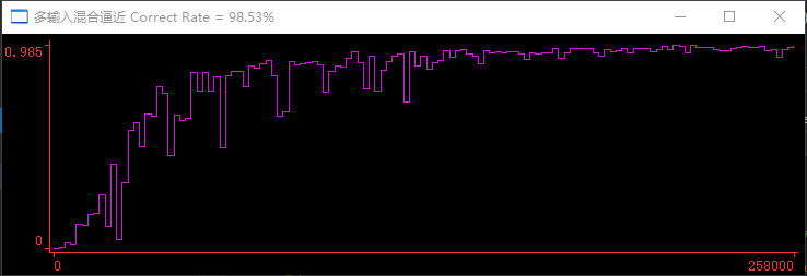
Net training epoch completed with achieve accuracy. CorrectRate(98.53%) >= TagCorrectRate(98.50%)
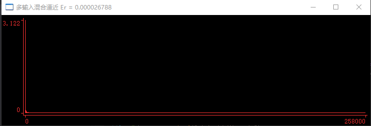
Epoch 5: total time: 38.3055 seconds, this time: 1.94778 seconds, correctrate = 98.53%, er = 2.6788e-05


Input value = {1.435037, 0.907074, 0.424992, - 0.815886,}
Predicted value = {- 0.728387, 0.911280, 0.252407, 0.806843,}
True value = {- 0.728333, 0.911042, 0.247706, 0.807685,}
Loss = 0.000011, < 0.0001 is predicted correctly!


Input value = {2.043433, - 0.558324, 1.185989, - 0.567262,}
Predicted value = {- 0.535745, 0.376521, 0.057957, 0.885794,}
True value = {- 0.537325, 0.375381, 0.057217, 0.885282,}
Loss = 0.000002, < 0.0001 is predicted correctly!


Input value = {- 0.058070, 2.371945, - 1.143344, 0.415305,}
Predicted value = {0.406086, 0.411661, 0.995162, 0.485440,}
True = {0.403469, 0.414554, 1.000000, 0.485487,}
Loss = 0.000019, < 0.0001 is predicted correctly!


Input value = {0.931005, - 1.908752, - 1.386756, - 2.818051,}
Predicted value = {- 0.318844, 0.182217, 0.014959, 0.718451,}
True value = {- 0.317927, 0.183003, 0.014827, 0.717279,}
Loss = 0.00000 1, < 0.0001 predicted correctly!


Input value = {2.984331, - 1.796760, - 2.753757, - 0.121948,}
Predicted value = {- 0.118123, - 0.923810, 0.018038, 0.951676,}
True = {- 0.121646, - 0.925730, 0.016584, 0.951861,}
Loss = 0.000009, < 0.0001 is predicted correctly!

Please press any key to continue