Experimental resources

1998.csv
airports.csv

Experimental environment

VMware Workstation
Ubuntu 16.04
spark-2.4.5
scala-2.12.10

Experimental content

"We are sorry to inform you that your flight XXXX from XX to XX has been delayed."
I believe many passengers waiting at the airport do not want to hear this sentence. With the gradual popularization of air transportation, the problem of flight delay has been perplexing us. Flight delays usually lead to two results, one is flight cancellation, the other is flight delay.
In this experiment, we will use DataFrame, SQL, machine learning framework and other tools provided by Spark, based on D3 JS data visualization technology, analyze the recorded data of flight take-off and landing, try to find out the causes of flight delay, and predict the flight delay.

Experimental steps

1, Data set introduction and preparation

1. Data set introduction

The flight data set used in this experiment is Statistics of flight punctuality rate provided on Data Expo in 2009 . This time we choose the data set of 1998.

The fields of this dataset are explained as follows:

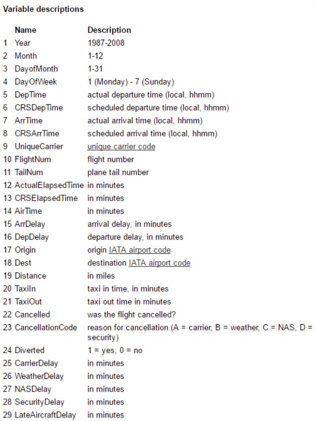
In addition, we will use some supplementary information. Such as airport information data set, etc.

2. Download dataset
(1) Enter the following command in the virtual machine

wget https://labfile.oss.aliyuncs.com/courses/610/1998.csv.bz2

(2) Then use the decompression command to decompress it

bunzip2 1998.csv.bz2

The extracted CSV data file is located in the working directory when you use the decompression command. By default, it is in the / home / user name directory.
(3) Similarly, download the airports airport information data set, and the command is as follows

wget https://labfile.oss.aliyuncs.com/courses/610/airports.csv

3. Data cleaning
Because the airports dataset contains some unusual characters, we need to clean them to prevent the unrecognizable errors of some recorded characters from causing subsequent retrieval errors.
OpenRefine is an open source data cleaning tool developed by Google. Let's install it in the environment first:

wget https://labfile.oss.aliyuncs.com/courses/610/openrefine-linux-3.2.tar.gz
tar -zxvf openrefine-linux-3.2.tar.gz
cd openrefine-3.2
# Start command
./refine

When the prompt message shown in the figure below appears, open the URL in the browser http://127.0.0.1:3333/ .

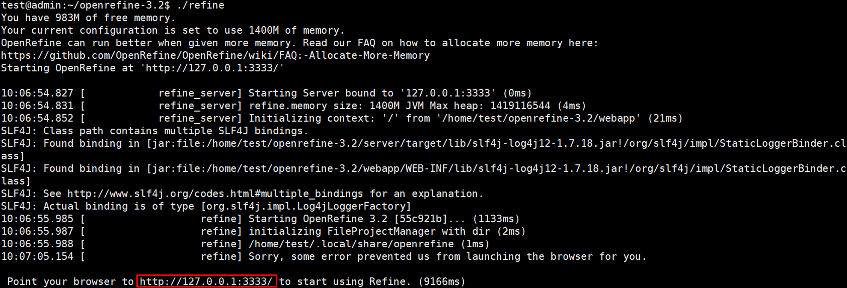
The successful start of Open Refine is marked by the appearance of Point your browser to http://127.0.0.1:3333 to start using Refine.
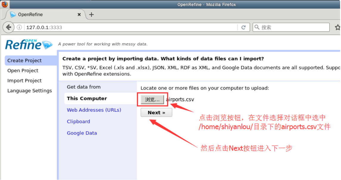
The application web page of OpenRefine will appear in the browser, as shown in the following figure. Please select the airport information data set just downloaded and click the Next button to enter the Next step.

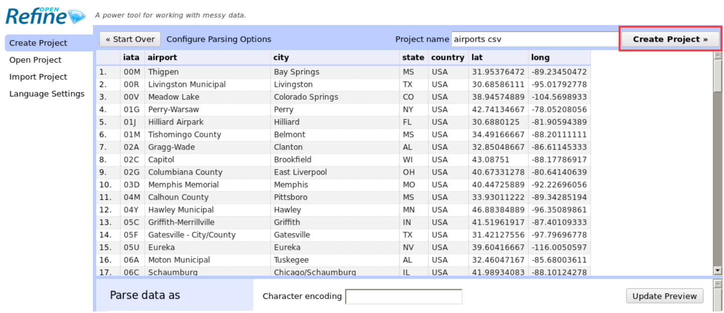
In the data analysis step, directly click the Create Project button in the upper right corner to create a data cleaning project.

After a short wait, you can perform various operations on the data after the project is created. A detailed tutorial on OpenRefine will be provided later. Here, you only need to follow the prompts to operate the dataset accordingly.
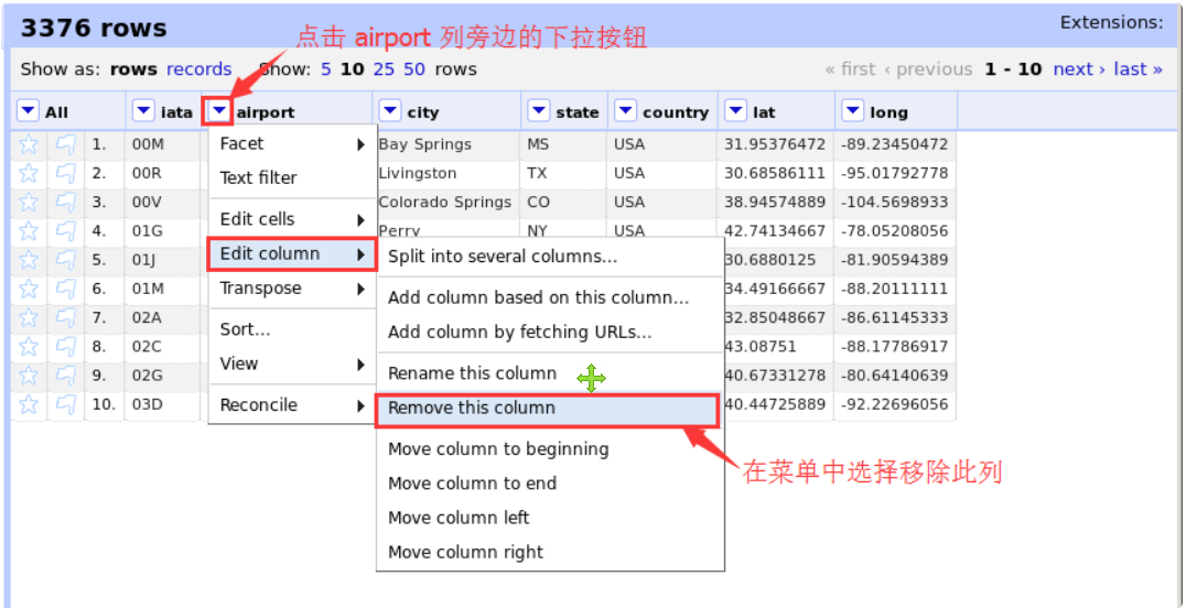
Click the drop-down menu button next to the airport column, and then select the edit column - > remove this column option in the menu to remove the airport column. The specific operation is shown in the figure below.

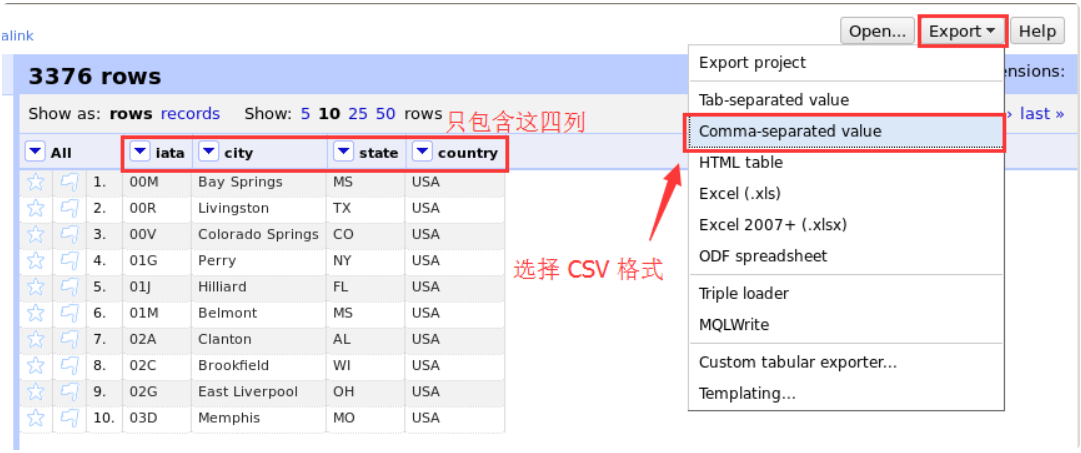
In the same way, remove the lat and long columns. The final dataset should contain only four columns: iata, city, state and country.
Finally, we click the Export button in the upper right corner to export the dataset. Select comma separated value as the export option, that is, CSV file.

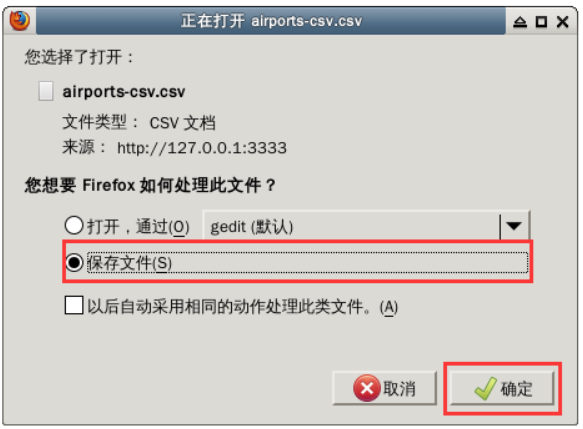
Then select "save file" in the pop-up download prompt dialog box and confirm.

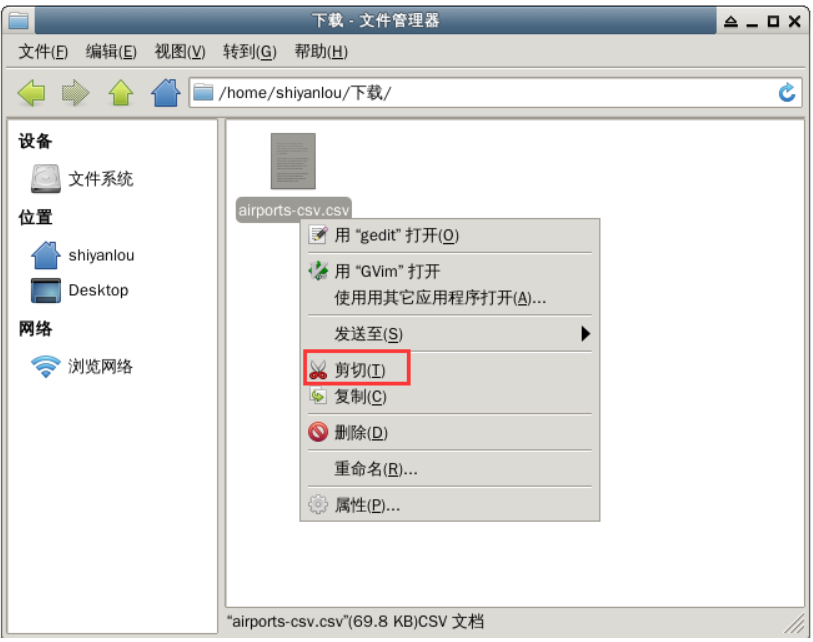
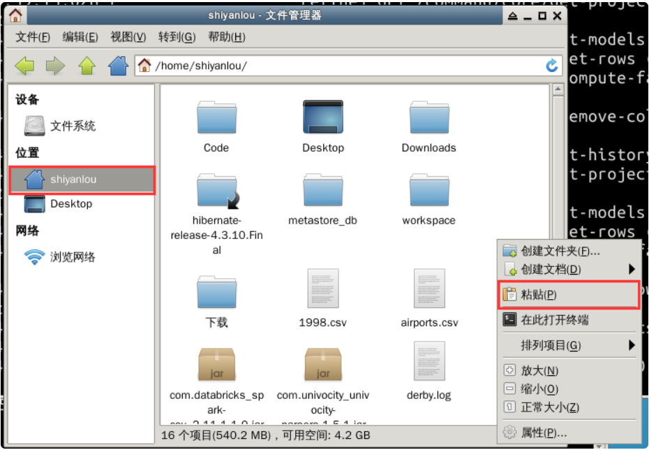
The file is located in the / home / user name / download directory. Please cut it to the / home / user name directory in the file manager and overwrite the source file. The steps are shown in the figure below.
First, double-click to open the home folder on the desktop and find the download directory. Right click the CSV file and select cut.

Then return to the main directory, right-click in the blank space and select "paste".

Finally, close the browser and the terminal running OpenRefine.

4. Start Spark Shell
In order to better handle the data set in CSV format, we can directly use the third-party Spark CSV parsing library provided by DataBricks company to read it.
The first is to start Spark Shell. At the same time of startup, attach the parameter -- packages com databricks:spark-csv_ 2.11:1.1.0

spark-shell --packages com.databricks:spark-csv_2.11:1.1.0

5. Import data and processing format
After the Spark Shell is started, enter the following command to import the dataset.

val sqlContext = new org.apache.spark.sql.SQLContext(sc)
val flightData = sqlContext.read.format("com.databricks.spark.csv").option("header","true").load("/home/shiyanlou/1998.csv")

In the above command, we call the read interface provided by sqlContext and specify that the loading format format is the format defined in the third-party library com databricks. spark. csv . At the same time, a read option is set, and the header is true, which means that the content of the first row in the dataset is resolved to the field name. Finally, the load method indicates that the data set file to be read is the data set we just downloaded.

At this time, the data type of flightData is DataFrame commonly used in Spark SQL. Register flightData as a temporary table. The command is:

flightData.registerTempTable("flights")

Use the same method to import the airport information dataset airports CSV and register it as a temporary table.

val airportData = sqlContext.read.format("com.databricks.spark.csv").option("header","true").load("/home/shiyanlou/airports-csv.csv")
airportData.registerTempTable("airports")

2, Data exploration

1. Problem design
Before exploring the data, we already know that the data has a total of 29 fields. Based on the departure time, departure / arrival delay and other information, we can boldly ask the following questions:

• **What are the busiest periods of flights every day** It is usually easy to have extreme weather such as heavy fog in the morning and evening. Are there more arrival and departure flights at noon?
• **Where is the most punctual flight** When designing the travel plan, if there are two adjacent airports to reach a certain destination, it seems that we can compare where it is more punctual, so as to reduce the impact of possible delays on our travel.
• **What are the hardest hit areas with delayed departure** Similarly, where are the most vulnerable to delays? The next time you start from these places, you should consider whether you want to change to ground transportation.

2. Problem solving
We have registered the data as a temporary table, and the answer to the above problem actually becomes how to design appropriate SQL query statements. When the amount of data is very large, Spark SQL is particularly convenient to use. It can directly pull data from distributed storage systems such as HDFS for query, and maximize the use of cluster performance for query calculation.
(1) What are the busiest periods of flights every day
When analyzing a question, we should find ways to implement the source of the answer to the question on each index of the data set. When the question is not detailed enough, you can take some representative values as the answer to the question.

For example, flights are divided into arrival and departure flights. If the number of departure flights of all airports in a certain period of time every day is counted, it can reflect whether the flights in this period are busy in a certain procedure.

Every record in the data set simply reflects the basic situation of the flight, but they do not directly tell us what happens every day and every time period. In order to get the latter information, we need to filter and count the data.

Therefore, we will naturally use statistical functions such as AVG (average), COUNT (COUNT) and SUM (SUM).

In order to count the number of flights by time period, we can roughly divide the time of the day into the following five periods:

• Early morning (00:00 - 06:00): most people are resting during this period, so we can reasonably assume that there are fewer flights during this period.
• Morning (06:01 - 10:00): some morning classes choose to start at this time, and the airport usually gradually enters the peak from this time.
• Noon (10:01 - 14:00): people starting from their residence in the morning usually arrive at the airport at this time, so there may be more flights starting at this time.
• Afternoon (14:01 - 19:00): similarly, it's more convenient to start in the afternoon. It's just in the evening when you arrive at your destination, but it's not too late. It's convenient to find a place to stay.
• Evening (19:01 - 23:59): at the end of the day, there may be fewer flights near the early morning.

When the data we need is not a single discrete data but based on a certain range, we can use the keyword BETWEEN x AND y to set the start and end range of the data.

With the above preparation, we can try to write the total number of flights with departure time between 0:00 and 6:00. The first selected target is the flights table, that is, FROM flights. The total number of flights can be counted on FlightNum (using the COUNT function), that is, COUNT(FlightNum). The limited condition is that the departure time is between 0 (representing 00:00) and 600 (representing 6:00), that is, WHERE DepTime BETWEEN 0 AND 600. So what we want to write is:

val queryFlightNumResult = sqlContext.sql("SELECT COUNT(FlightNum) FROM flights WHERE DepTime BETWEEN 0 AND 600")

View one of the results:

queryFlightNumResult.take(1)

On this basis, we can refine it, calculate the average number of departure flights per day, and select only one month's data each time. Here we choose the time period from 10:00 to 14:00.

// COUNT(DISTINCT DayofMonth) is used to calculate the number of days in each month
val queryFlightNumResult1 = sqlContext.sql("SELECT COUNT(FlightNum)/COUNT(DISTINCT DayofMonth) FROM flights WHERE Month = 1 AND DepTime BETWEEN 1001 AND 1400")

There is only one query result, that is, the average number of departing flights per day in that month. Check:

queryFlightNumResult1.take(1)

You can try to calculate the average number of departure flights in other time periods and keep records.
The final statistical results show that in January 1998, the busiest time of day was afternoon. The average number of departing flights in this period is 4356.7.
(2) Where is the most punctual flight
It depends on which flight is the most punctual. In fact, it is to count the arrival on time rate of flights. You can check where the flights with arrival delay time of 0 go first.
In the above sentence, there are several messages:

• The main information to be queried is the destination code.
• The source of information is the flights table.
• The arrival time of the query condition of arr0 is delay.

In the face of any problem, we can follow the above ideas to disassemble the problem, and then convert each piece of information into the corresponding SQL statement.

So we can finally get such a query code:

val queryDestResult = sqlContext.sql("SELECT DISTINCT Dest, ArrDelay FROM flights WHERE ArrDelay = 0")

Take out five of the results and have a look.

queryDestResult.head(5)

On this basis, we try to add more restrictions.

We can count the number of arrival flights with delay time of 0 (on-time times), and the final output result is [destination, on-time times], and arrange them in descending order.

val queryDestResult2 = sqlContext.sql("SELECT DISTINCT Dest, COUNT(ArrDelay) AS delayTimes FROM flights where ArrDelay = 0 GROUP BY Dest ORDER BY delayTimes DESC")

View 10 of the results.

queryDestResult2.head(10)

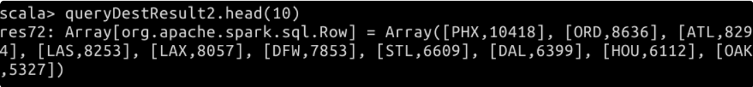
In the United States, a state usually has multiple airports. The query results obtained in the previous step are output according to the airport code of the destination. So how many arriving flights are there in every state on time?

Based on the previous query, we can perform nested query again. In addition, we will use the information in another data set airports: the three word code (Dest) in the destination is the iata code (iata) in the data set, and each airport gives the information (state) of its state. We can add the airports table to the query through a join operation.

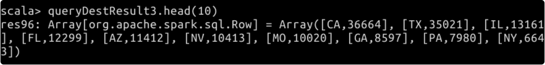
val queryDestResult3 = sqlContext.sql("SELECT DISTINCT state, SUM(delayTimes) AS s FROM (SELECT DISTINCT Dest, COUNT(ArrDelay) AS delayTimes FROM flights WHERE ArrDelay = 0 GROUP BY Dest ) a JOIN airports b ON a.Dest = b.iata GROUP BY state ORDER BY s DESC")

View 10 of the results.

queryDestResult3.head(10)

Finally, you can also output the results in CSV format and save them in the user's home directory.

// QueryDestResult.csv is just the name of the folder where the results are saved
queryDestResult3.rdd.saveAsTextFile("/home/shiyanlou/QueryDestResult.csv")

After saving, we also need to manually merge it into one file. Open a new terminal and enter the following command in the terminal to merge files.

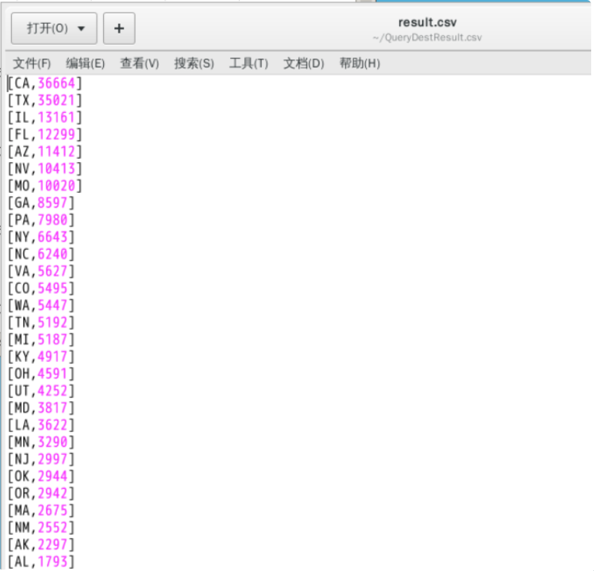
# Enter the directory of the result file
cd ~/QueryDestResult.csv/

# Use wildcards to append the contents of each part file to result CSV file
cat part-* >> result.csv

Finally, open result The final result can be seen in the CSV file, as shown in the figure below.

(3) What are the hardest hit areas with delayed departure
You can boldly set the query condition that the departure delay is greater than 60 minutes, and write the query statement as follows:

val queryOriginResult = sqlContext.sql("SELECT DISTINCT Origin, DepDelay FROM flights where DepDelay > 60 ORDER BY DepDelay DESC")

Because the data has been arranged in descending order, we take out the first 10 query results, that is, the ten flights with the most serious delays and the departure airport in 1998.

queryOriginResult.head(10)

3, Flight delay time prediction

1. Introduction

Historical data is a record of what has happened in the past. We can summarize the past according to historical data. So can we look forward to the future according to this?

Maybe the first thing you think of is prediction. When it comes to prediction, we have to mention one of the most popular disciplines - machine learning. Prediction is also one of the tasks that machine learning related knowledge can complete.

As data analysts, the main purpose of learning machine learning is not to improve the machine learning algorithm in all aspects (machine learning experts are working hard for this). The minimum requirement should be to be able to apply the machine learning algorithm to practical data analysis problems.

2. Introduce related packages

import org.apache.spark._
import org.apache.spark.rdd.RDD
import org.apache.spark.mllib.util.MLUtils
import org.apache.spark.mllib.linalg.Vectors
import org.apache.spark.mllib.regression.LabeledPoint
import org.apache.spark.mllib.tree.DecisionTree
import org.apache.spark.mllib.tree.model.DecisionTreeModel

3. Convert DataFrame to RDD

Most operations in Spark ML are based on RDD (distributed elastic data set). The data type of the data set we read in before is DataFrame. Each record in the DataFrame corresponds to each row value in the RDD. To do this, we need to convert the DataFrame to RDD.

First, the data is converted from DataFrame type to RDD type. When taking values from row, the value of the corresponding field in Flight class is taken out according to each field in the dataset. For example, row(3) in the second row takes out the value of DayOfWeek field in DataFrame, which corresponds to DayOfWeek member variable in Flight class.

val tmpFlightDataRDD = flightData.map(row => row(2).toString+","+row(3).toString+","+row(5).toString+","+row(7).toString+","+row(8).toString+","+row(12).toString+","+ row(16).toString+","+row(17).toString+","+row(14).toString+","+row(15).toString).rdd

Next, you need to create a class to map some fields in RDD to the member variables of the class.

case class Flight(dayOfMonth:Int, dayOfWeek:Int, crsDepTime:Double, crsArrTime:Double, uniqueCarrier:String, crsElapsedTime:Double, origin:String, dest:String, arrDelay:Int, depDelay:Int, delayFlag:Int)

In Flight class, the last member variable is delayFlag. Through the observation of the data, we know that the delay time of some flights is only a few minutes (whether on departure or arrival), and usually such delay is tolerable. In order to reduce the amount of data to be processed, we can define the delay as the delay time of departure or arrival is greater than half an hour (i.e. 30 minutes), so as to simplify the arrival delay time and departure delay time into delay flag.

You can try to write pseudo code first:

if ArrDelayTime or DepDelayTime > 30
    delayFlag = True
else
    delayFlag = False

Then we define an analysis method according to the above logic. This method is used to convert records in DataFrame to RDD.

def parseFields(input: String): Flight = {
    val line = input.split(",")

    // Filter for possible invalid value "NA"
    var dayOfMonth = 0
    if(line(0) != "NA"){
        dayOfMonth = line(0).toInt
    }
    var dayOfWeek = 0
    if(line(1) != "NA"){
        dayOfWeek = line(1).toInt
    }

    var crsDepTime = 0.0
    if(line(2) != "NA"){
        crsDepTime = line(2).toDouble
    }

    var crsArrTime = 0.0
    if(line(3) != "NA"){
        crsArrTime = line(3).toDouble
    }

    var crsElapsedTime = 0.0
    if(line(5) != "NA"){
        crsElapsedTime = line(5).toDouble
    }

    var arrDelay = 0
    if(line(8) != "NA"){
        arrDelay = line(8).toInt
    }
    var depDelay = 0
    if(line(9) != "NA"){
        depDelay = line(9).toInt
    }

    // Determine whether the delay flag is 1 according to the delay time
    var delayFlag = 0
    if(arrDelay > 30 || depDelay > 30){
        delayFlag = 1
    }
    Flight(dayOfMonth, dayOfWeek, crsDepTime, crsArrTime, line(4), crsElapsedTime, line(6), line(7), arrDelay, depDelay, delayFlag)
}

After the definition of the parsing method is completed, we use the map operation to parse the fields in the RDD.

val flightRDD = tmpFlightDataRDD.map(parseFields)

You can try to randomly fetch a value to check whether the parsing is successful.

flightRDD.take(1)

4. Extract features

In order to establish the classification model, we need to extract the features of flight data. In the step of parsing data just now, we set delayFlag to define two classes for classification. Therefore, you can call it Label, which is a common means in classification. There are two kinds of tags. If delayFlag is 1, it means that the flight is delayed; If it is 0, it means there is no delay. The criterion for distinguishing delay is as discussed earlier: whether the delay in arrival or departure exceeds 30 minutes.

For each record in the dataset, they now contain label and characteristic information. The feature is all attributes corresponding to each record in the Flight class (from dayOfMonth to delayFlag).

Next, we need to convert these features into numerical features. In the Flight class, some attributes are already numerical characteristics, while attributes such AS crsDepTime and uniqueCarrier are not numerical characteristics. In this step, we have to convert them into numerical features. For example, the uniqueCarrier feature is usually the airline code ("WN" and so on). We number them in sequence and convert the string type feature into a numerical feature with unique ID (for example, "AA" becomes 0, "AS" becomes 1, and so on. The actual operation is marked in alphabetical order).

var id: Int = 0
var mCarrier: Map[String, Int] = Map()
flightRDD.map(flight => flight.uniqueCarrier).distinct.collect.foreach(x => {mCarrier += (x -> id); id += 1})

After the calculation, let's check whether the conversion from the string representing the airline code to the corresponding unique ID has been completed in the carrier.

mCarrier.toString

According to the same logic, we need to convert string to value for Origin and Dest.

First, convert Origin:

var id_1: Int = 0
var mOrigin: Map[String, Int] = Map()
// The origin here is equivalent to a "global" variable, and we are modifying it in every map

flightRDD.map(flight => flight.origin).distinct.collect.foreach(x => {mOrigin += (x -> id_1); id_1 += 1})

The last is to convert Dest. Don't forget that the purpose of our conversion is to establish numerical features.

var id_2: Int = 0
var mDest: Map[String, Int] = Map()
flightRDD.map(flight => flight.dest).distinct.collect.foreach(x => {mDest += (x -> id_2); id_2 += 1})

So far, we have all the features ready.

5. Define feature array

In the previous step, we used different numbers to represent different features. These features will finally be put into the array, which can be understood as establishing the feature vector.

Next, we store all tags (delay or not) and features in a new RDD in numerical form as input to the machine learning algorithm.

val featuredRDD = flightRDD.map(flight => {
  val vDayOfMonth = flight.dayOfMonth - 1
  val vDayOfWeek = flight.dayOfWeek - 1
  val vCRSDepTime = flight.crsDepTime
  val vCRSArrTime = flight.crsArrTime
  val vCarrierID = mCarrier(flight.uniqueCarrier)
  val vCRSElapsedTime = flight.crsElapsedTime
  val vOriginID = mOrigin(flight.origin)
  val vDestID = mDest(flight.dest)
  val vDelayFlag = flight.delayFlag

  // In the return value, all fields are converted to Double type to facilitate the use of relevant API s during modeling
  Array(vDelayFlag.toDouble, vDayOfMonth.toDouble, vDayOfWeek.toDouble, vCRSDepTime.toDouble, vCRSArrTime.toDouble, vCarrierID.toDouble, vCRSElapsedTime.toDouble, vOriginID.toDouble, vDestID.toDouble)
})

After going through the map stage, we get all the features of the array.

Try to fetch one of the values to see if the conversion was successful.

featuredRDD.take(1)

6. Create marker points

In this step, we need to convert the featuredRDD containing the feature array to org apache. spark. mllib. regression. The new RDD of the marker points LabeledPoints defined in the labeledpoint package. In classification, marker points contain two types of information: one represents the marker of data points, and the other represents the feature vector class.

Let's finish this conversion.

// Label is set to DelayFlag, and Features is set to the values of all other fields
val LabeledRDD = featuredRDD.map(x => LabeledPoint(x(0), Vectors.dense(x(1), x(2), x(3), x(4), x(5), x(6), x(7), x(8))))

Try to fetch one of the values to see if the conversion was successful.

LabeledRDD.take(1)

Review the previous work: we got the data with delay flag. All flights can be marked as delayed or no delay. Next, we will use the random division method to divide the above data into training set and test set.

The following is a detailed description of the scale:

• In LabeledRDD, the data marked with DelayFlag = 0 is non delayed flight; The data marked with DelayFlag = 1 is the delayed flight.

• 80% of the total number of non delayed flights will form a new data set with all delayed flights. 70% and 30% of the new data set will be divided into training set and test set.

• The purpose of not directly using the data in LabeledRDD to divide the training set and test set is to improve the proportion of delayed flights in the test set as much as possible, so that the trained model can more accurately describe the delay.

Therefore, we first extract all non delayed flights in LabeledRDD, and then randomly extract 80% of them.

// (0) at the end is to take the 80% part
val notDelayedFlights = LabeledRDD.filter(x => x.label == 0).randomSplit(Array(0.8, 0.2))(0)

Then we extract all the delayed flights.

val delayedFlights = LabeledRDD.filter(x => x.label == 1)

The above two are combined into a new data set for subsequent division of training set and test set.

val tmpTTData = notDelayedFlights ++ delayedFlights

Finally, we randomly divide the data set into training set and test set according to the agreed proportion.

// TT means train & test
val TTData = tmpTTData.randomSplit(Array(0.7, 0.3))
val trainingData = TTData(0)
val testData = TTData(1)

7. Training model

Next, we will extract features from the training set. The in Spark MLlib will be used here Decision tree . Decision tree is a prediction model, which represents a mapping relationship between object attributes and object values. You can Baidu Encyclopedia Learn the principle of decision tree in detail.

I hope you can use some time to understand the decision tree before proceeding with the next work, so as to better understand the meaning of various parameter settings.

In the official documents, the parameters of the decision tree are divided into three categories:

• Problem specification parameters: these parameters describe the problem to be solved and the data set. We need to set categorialfeaturesinfo, which indicates which features have been defined and how many explicit values these features can take. The return value is a Map. For example, Map (0 - > 2, 4 - > 10) indicates that there are 2 values (0 and 1) for feature 0 and 10 values (from 0 to 9) for feature 4.

• Stopping criteria: these parameters determine when the construction of the tree stops (that is, stop adding new nodes). We need to set maxDepth, which represents the maximum depth of the tree. A deeper tree may be more expressive, but it is also more difficult to train and easier to over fit.

• Tunable parameters: these parameters are optional. We need to set two. The first is maxBins, which represents the amount of bucket information when discrete continuous features are used. The second is impurity, which indicates the impurity degree when selecting candidate branches.

The model we want to train is to establish the relationship between the input characteristics and the marked output. The method to be used is the trainClassifier method of decision tree class DecisionTree. By using this method, we can get a decision tree model.

Let's try to construct training logic.

// Follow the tips in the API document to construct various parameters
var paramCateFeaturesInfo = Map[Int, Int]()

// The first feature information: the subscript is 0, indicating that dayOfMonth has a value from 0 to 30.
paramCateFeaturesInfo += (0 -> 31)

// The second feature information: the subscript is 1, indicating that dayOfWeek has a value from 0 to 6.
paramCateFeaturesInfo += (1 -> 7)

// The third and fourth features are departure and arrival time, which we will not use here, so it is omitted.

// The fifth feature information: the subscript is 4, indicating all values of uniqueCarrier.
paramCateFeaturesInfo += (4 -> mCarrier.size)

// The sixth characteristic information is flight time, which is also ignored.

// The seventh feature information: the subscript is 6, indicating all values of origin.
paramCateFeaturesInfo += (6 -> mOrigin.size)

// The eighth characteristic information: subscript 7 indicates all values of dest.
paramCateFeaturesInfo += (7 -> mDest.size)

// The number of categories is 2, representing delayed flights and non delayed flights.
val paramNumClasses = 2

// The following parameters are set to empirical values
val paramMaxDepth = 9
val paramMaxBins = 7000
val paramImpurity = "gini"

After the parameter construction is completed, we call trainclassifier method for training.

val flightDelayModel = DecisionTree.trainClassifier(trainingData, paramNumClasses, paramCateFeaturesInfo, paramImpurity, paramMaxDepth, paramMaxBins)

After the training, we can try to print out the decision tree.

val tmpDM = flightDelayModel.toDebugString
print(tmpDM)

The execution results are shown in the figure below. All results are not displayed here.

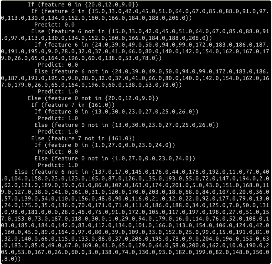
The content of the decision tree looks like a multi branch structure. If you have enough patience, you can draw the conditions of the decision one by one on the draft paper. According to the above conditions, we can predict an input value in the future. Of course, the result of the prediction is that there will be delay or no delay.

8. Test model

After the model training, we also need to test the construction effect of the model. Therefore, the final step is to test the model with the test set.

// The predict method of decision tree model is used to predict according to the input, and the prediction results are temporarily stored in tmpPredictResult. Finally, it forms Yuanzu with the mark of input information as the final return result.
val predictResult = testData.map{flight =>
  val tmpPredictResult = flightDelayModel.predict(flight.features)
  (flight.label, tmpPredictResult)
}

Try to take out 10 groups of prediction results and see the effect.

predictResult.take(10)

The execution results are shown in the figure below.

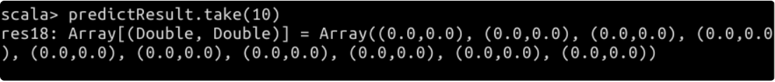
It can be seen that if 0.0 of Label corresponds to 0.0 of PredictResult, the prediction result is correct. And not every prediction is accurate.

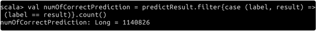
val numOfCorrectPrediction = predictResult.filter{case (label, result) => (label == result)}.count()

The execution results are shown in the figure below.

Finally, calculate the accuracy of prediction:

// toDouble is used to improve the accuracy of accuracy. Otherwise, the division of two long values is still a long value.
val predictAccuracy = numOfCorrectPrediction/testData.count().toDouble

The execution results are shown in the figure below.

We get that the prediction accuracy of the model is about 85.77%. It can be said that it has certain application value in practical prediction. In order to improve the accuracy of prediction, you can consider using more data for model training, and adjust the parameters to the best when building the decision tree.

Because the data set will be different in each random division process, the prediction accuracy here is for reference only. If the result is more than 80%, it can be regarded as the goal of the project.

9,D3.js visual programming

The purpose of data visualization is to make the data more credible. If we stare at a pile of tables and figures, we are likely to ignore some important information. As an expression of data, data visualization can help us find some information that is not easy to see from the data surface.

In fact, before that, we have been more or less exposed to data visualization. The simplest data visualization is the histogram, line chart, pie chart and so on we make in Microsoft Office Excel. Data visualization is not about how cool the charts are, but how to express complex data more vividly.

The full name of D3 is Data-Driven Documents, which literally means Data-Driven Documents. It itself is a JavaScript function library, which can be used for data visualization.

Let's use a lightweight example to learn how to show the number of on-time flights in each state and their overall busyness on the map of the United States.

(1) Create project directories and files

Double click on the desktop to open the terminal and download D3 required for the course JS and other javascript script files.

wget https://labfile.oss.aliyuncs.com/courses/610/js.tar.gz

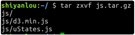
Then decompress it.

tar zxvf js.tar.gz

Now let's create the directories and files needed for the project. First, create a new project directory called DataVisualization. All web pages, js files and data are stored in this directory.

mkdir DataVisualization

Enter the newly created directory, create two directories named data and js respectively to store CSV data and js files, and finally create another directory named index HTML web page file.

cd DataVisualization
mkdir data
mkdir js
touch index.html

The data for data visualization comes from the data we save in / home / shiyanlou / querydestresult Result in CSV / directory CSV file. We copy it to the data folder under the current project directory.

cp ~/QueryDestResult.csv/result.csv ~/DataVisualization/data

For the whole project, we need to be in index Calling D3. in html web page js to write the main data visualization logic. And corresponding html elements will be added to display the data visualization results. Therefore, we also need to copy the two js files extracted before to the js folder of the project directory.

cp ~/js/* ~/DataVisualization/js

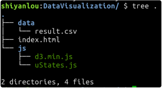
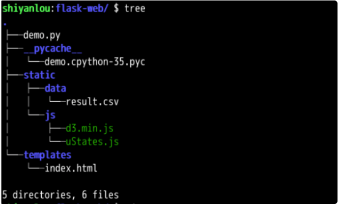
Finally, we use the tree command to view the file structure of the project directory.

tree .

(2) Data completeness check

First, remove result Brackets at the beginning and end of each line in CSV file:

sed -i "s/\[//g" ~/DataVisualization/data/result.csv
sed -i "s/\]//g" ~/DataVisualization/data/result.csv

Usually, drawing is prone to errors because the data contains invalid or missing values.

There are two ways to avoid such errors: one is to carry out fault-tolerant processing through programs; The second is to check the completeness of the data and make up the invalid or missing values.

For simplicity, we revise the data directly through the text editor.

Please use gedit text editor to open the data file.

gedit ~/DataVisualization/data/result.csv

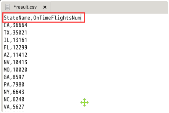
The first step is to add field names to the CSV file. Please add fields to the two columns of data in the first row: StateName and ontimeflightnum. The details are shown in the figure below (pay attention to case).

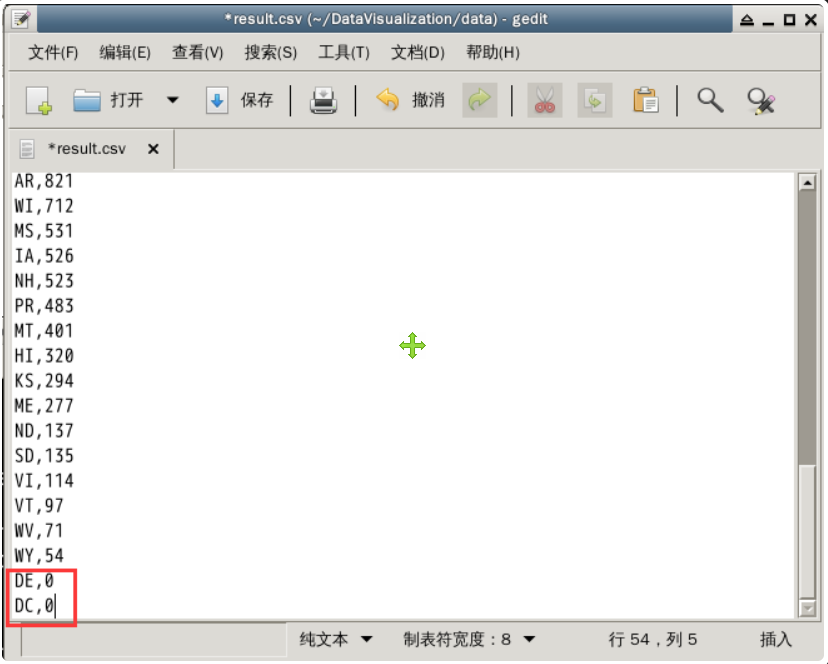
Comparing with the list of state names in the United States, we can find result The information of Washington, D.C. (DC) and Delaware (DE) is still missing in CSV. We add them at the end of the file and set the number of on-time flights to 0, as shown in the figure below.

(3) Edit index html

index. In HTML, we need to insert some basic HTML elements to make it look more "like" a web page.

Please check the index Add the following content to HTML.

<!DOCTYPE html>
<html>
    <head>
        <meta charset="utf-8">
        <title>US OnTime Flights Map</title>
    </head>
    <body>
    </body>
</html>

Because we use D3 JS, so it needs to be referenced in HTML code here. In addition, we also need one called ustates JS, which already contains the contour data of various states in the United States.

Please insert the following statement between < head > tags to reference the corresponding js file.

The inserted code is:

        <script src="js/d3.min.js"></script>
        <script src="js/uStates.js"></script>

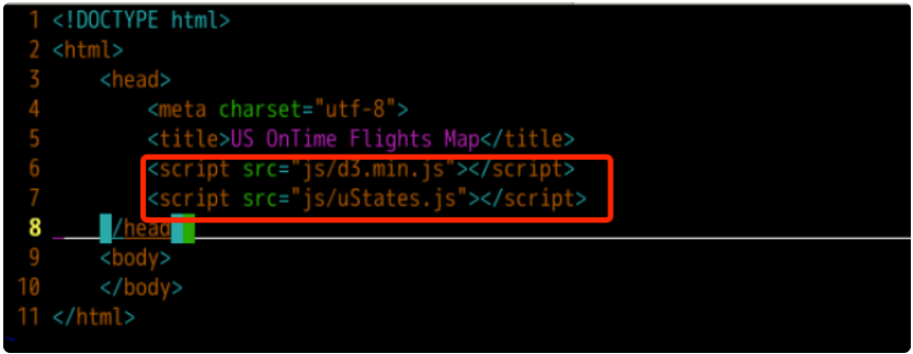
We set the source of the js file in the src attribute to the corresponding js file in the js directory under the root directory of the web page.

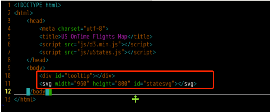
After that, we need to insert some HTML elements between < body > tags.

In the following code, the svg tag is used to display the map of the United States, and the div tag is used to load the relevant information of the prompt box. We set the id of the element where the prompt box is located as tooltip, the id of the element where the map is located as statesvg, and the width and height are 960 and 800 pixels respectively.

    <!-- Should div The label is used to load the prompt box -->
    <div id="tooltip"></div>
    <!-- SVG Labels are used to draw maps -->
    <svg width="960" height="800" id="statesvg"></svg>

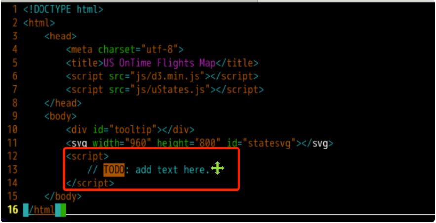
Finally, we need to prepare a script tag to write the logic code related to our data visualization.

Please insert the following between the < body > tags.

    <script>
    </script>

(4) Realize the relevant functions of data loading and visual preparation

The first step is to read the data from the CSV file. Here we directly use D3 JS API function D3 csv().

In this function, the first parameter is the file path to be read. We set it as data / result CSV, which represents the result in the data directory under the project directory CSV file.

The second parameter is the anonymous callback function after reading, that is, the contents of the callback function will be executed after reading (whether successful or not). Error and csvData are two parameters that must be passed. When reading fails, we can use console Log (error) is used to output error information on the browser console. When the reading is successful, csvData is the variable loaded with the contents of the CSV file.

Please insert the following code into the added script tag.

d3.csv("data/result.csv", function(error, csvData) {
    // TODO: add text here.
});

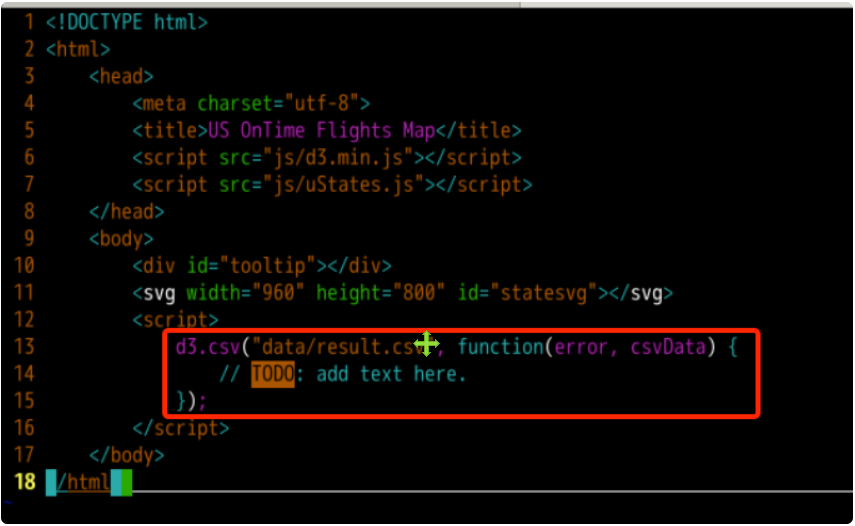
Everything we need to do later will be completed in this callback function.

For convenience, we will continue to explain the relevant knowledge points in the notes.

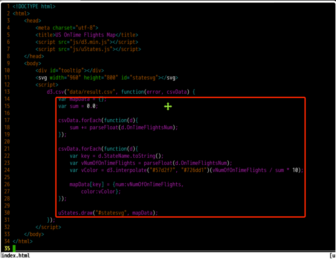
You need to insert the callback function into the following code.

// Create an Object to store the processed drawing data
// It can be understood as a map object containing key - value
var mapData = {};

// The variable sum is used to store the total number of on-time flights
var sum = 0.0;

// Traverse csvData for the first time to calculate the total number of punctual flights
csvData.forEach(function(d){
    // In the forEach function, an anonymous function is used to process the data records obtained from each traversal d
    // OnTimeFlightsNum is the name of the field we set in the CSV file
    // The retrieved value is still of string type. We need to convert it to floating point
    sum += parseFloat(d.OnTimeFlightsNum);
});

// The second traversal of csvData is used to set the drawing data
csvData.forEach(function(d){

    // d.StateName takes out the value of the StateName field of each record and converts it into a string as the key of the map object
    var key = d.StateName.toString();

    // d.OnTimeFlightsNum takes out the value of OnTimeFlightsNum field of each record and converts it to floating-point type
    var vNumOfOnTimeFlights = parseFloat(d.OnTimeFlightsNum);

    // Here is to set different levels of color for different data
    // D3 was called JS interpolation API: D3 interpolate()
    // Parameters "#57d2f7" and "#726dd1" are HEX type hexadecimal color codes, and each two bits are the color depth of RGB channel respectively
    // Use vNumOfOnTimeFlights / sum to calculate the proportion of the current value in the total, and multiply by 10 to make the color discrimination more obvious
    var vColor = d3.interpolate("#57d2f7", "#726dd1")(vNumOfOnTimeFlights / sum * 10);

    // For each record, the value of the StateName field is used as the key of mapData, and the number of on-time flights and color code are used as their values.
    mapData[key] = {num:vNumOfOnTimeFlights,
        color:vColor};
});


// When the drawing data is ready, the draw function of the uStates object is invoked for drawing.
// The first parameter is the selected drawing object, that is, the HTML tag we set: statesvg
// The second parameter is the plot data we calculated
uStates.draw("#statesvg", mapData);

The completed code is shown in the figure below.

(5) Implement ustates Drawing function in JS

In index The data needed for drawing is calculated in HTML, and finally the draw function of uStates object is called. Here we need to improve the logic of this drawing.

Now edit js / ustates js file, which is a js file prepared for you in advance. We need to improve some details.

In the current code, a lot of content is the definition of the variable uStatePaths. In this map, id is the abbreviation of states in the United States. We will use it later to find the number of on-time flights and color codes in the mapping data mapData; n is the full name corresponding to each state, which will be placed in the prompt box displayed when the mouse crosses; d is the outline of each state on the map.

It should be further explained that the contour data stored in d comes from the SVG file made according to the map of the United States. The production steps are as follows: first, make projection according to the GeoJSON data (such as Google Map) provided by the map service provider. GeoJSON contains some longitude and latitude, posters and other information, and then use d3 The projection function of JS projects it (d3.geo.mercator()), which can be scaled and translated during the projection process. After projection, two-dimensional data are obtained, but they are all points. The contours of the map are closed lines, so we also need to use d3 JS path generator (d3.geo.path()) to link the two-dimensional data points of each block to form the final map outline.

Usually, we will store the contour data in SVG file, which means scalable vector graphics. In this example, in order to simplify the operation steps, the data is directly given to the information of each state, that is, the description information you see.

Turning to the end of this code, you can see ustates The details in the draw have not been completed yet, which is what needs to be done next.

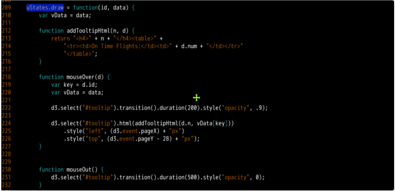
Please go to ustates draw = function (id, data) { ... }; The following contents are supplemented in the function definition of. Similarly, relevant explanations will be given in the form of notes.

// vData is used to load drawing data
var vData = data;

// This method is used to create the HTML content (div element) of the prompt box displayed when the mouse crosses
function addTooltipHtml(n, d) {
    // The incoming n is the full name of each state, represented by the h4 tag
    // D is the drawing data of each state, and d.num is the number of on-time flights
    return "<h4>" + n + "</h4><table>" +
        "<tr><td>On Time Flights:</td><td>" + d.num + "</td></tr>"
        "</table>";
}

// The mouseover event occurs when the mouse pointer is over the element
// A mouseOver function is defined here as the callback function for this event
function mouseOver(d) {
    // The d passed in is the element in uStatePaths
    var key = d.id;
    var vData = data;

    // Use D3 The select() function of JS selects the div element with id tooltip in the HTML element
    // The transition() function is used to start the transition effect and can be used for animation
    // duration(200) the duration used to animate is 200 milliseconds
    // Style ("Opacity",. 9) is used to set the opacity level of div elements. An opacity of. 9 means 90% opacity
    d3.select("#tooltip").transition().duration(200).style("opacity", .9);

    // Similarly, use the html() function to call the addTooltipHtml function to inject html code into the tooltip element
    // d.n represents the n member in sStatePaths, that is, the full name of each state
    // vData[key] means to use key to query the number of on-time flights of each state in the drawing data
    d3.select("#tooltip").html(addTooltipHtml(d.n, vData[key]))
        .style("left", (d3.event.pageX) + "px")
        .style("top", (d3.event.pageY - 28) + "px");
}


// The mouseout event occurs when the mouse pointer is no longer over the element
// A mouseOut function is defined here as the callback function for this event
function mouseOut() {
    // Setting the opacity to 0 is equivalent to making the div element disappear
    d3.select("#tooltip").transition().duration(500).style("opacity", 0);
}

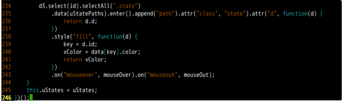
// The id here will soon represent the svgstate element
// This step sets the color for all States
// .data(uStatePaths).enter().append("path") means to draw a path using the data in ustatepaths
// . style("fill", function(d) {}) means to fill according to the color code of each state in the drawing data
// .on("mouseover", mouseOver).on("mouseout", mouseOut) indicates the listener and callback function for setting mouse coverage and mouse removal events
d3.select(id).selectAll(".state")
    .data(uStatePaths).enter().append("path").attr("class", "state").attr("d", function(d) {
        return d.d;
    })
    .style("fill", function(d) {
        key = d.id;
        vColor = data[key].color;
        return vColor;
    })
    .on("mouseover", mouseOver).on("mouseout", mouseOut);

The completed code is shown in the following figure:

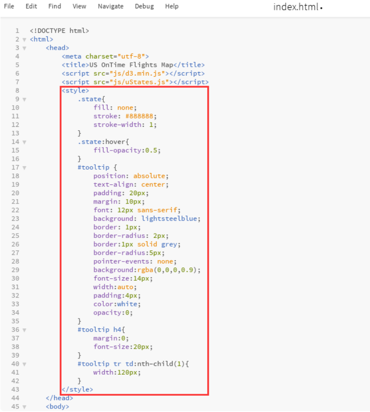
(6) Style page elements

Finally, we need to do some beautification work.

Back to index HTML, insert the following into the < head > tag.

<style>
    .state{
        fill: none;
        stroke: #888888;
        stroke-width: 1;
    }
    .state:hover{
        fill-opacity:0.5;
    }
    #tooltip {
        position: absolute;
        text-align: center;
        padding: 20px;
        margin: 10px;
        font: 12px sans-serif;
        background: lightsteelblue;
        border: 1px;
        border-radius: 2px;
        border:1px solid grey;
        border-radius:5px;
        pointer-events: none;
        background:rgba(0,0,0,0.9);
        font-size:14px;
        width:auto;
        padding:4px;
        color:white;
        opacity:0;
    }
    #tooltip h4{
        margin:0;
        font-size:20px;
    }
    #tooltip tr td:nth-child(1){
        width:120px;
    }
</style>

For the role of each attribute, please refer to W3school. The completed code is shown in the figure below.

So far, all our code editing work has been completed.

Final index The HTML page code is as follows:

<!DOCTYPE html>
<html>
    <head>
        <meta charset="utf-8">
        <title>US OnTime Flights Map</title>
        <script src="js/d3.min.js"></script>
        <script src="js/uStates.js"></script>
        <style>
            .state{
                fill: none;
                stroke: #888888;
                stroke-width: 1;
            }
            .state:hover{
                fill-opacity:0.5;
            }
            #tooltip {
                position: absolute;
                text-align: center;
                padding: 20px;
                margin: 10px;
                font: 12px sans-serif;
                background: lightsteelblue;
                border: 1px;
                border-radius: 2px;
                border:1px solid grey;
                border-radius:5px;
                pointer-events: none;
                background:rgba(0,0,0,0.9);
                font-size:14px;
                width:auto;
                padding:4px;
                color:white;
                opacity:0;
            }
            #tooltip h4{
                margin:0;
                font-size:20px;
            }
            #tooltip tr td:nth-child(1){
                width:120px;
            }
        </style>
    </head>
    <body>
        <div id="tooltip"></div>
        <svg width="960" height="800" id="statesvg"></svg>
        <script>
            d3.csv("data/result.csv", function(error, csvData) {
                var mapData = {};
                var sum = 0.0;

                csvData.forEach(function(d){
                    sum += parseFloat(d.OnTimeFlightsNum);
                });

                csvData.forEach(function(d){
                    var key = d.StateName.toString();
                    var vNumOfOnTimeFlights = parseFloat(d.OnTimeFlightsNum);
                    var vColor = d3.interpolate("#57d2f7", "#726dd1")(vNumOfOnTimeFlights / sum * 10);

                    mapData[key] = {num:vNumOfOnTimeFlights,
                        color:vColor};
                });

                uStates.draw("#statesvg", mapData);
            });
        </script>
    </body>
</html>

(7) Project Preview

Because the static page cannot read the local file, open index.com directly HTML page cannot view the page content. Here we simply use flash to start a service.

Flash has been installed in the experimental environment, and we can use it directly.

Create a new flash web folder in the / home/shiyanlou directory and enter the folder to create a new demo Py file, static folder and templates folder, and copy the contents in the DataVisualization folder. The final file directory structure is as follows:

In demo Write the following code in the PY file:

from flask import Flask
from flask import render_template
app = Flask(__name__)

@app.route('/')
def home():
    return render_template("index.html")

And modify the index HTML path. The main modifications are as follows:

        <script src="../static/js/d3.min.js"></script>
        <script src="../static/js/uStates.js"></script>
        ...
            d3.csv("/static/data/result.csv", function(error, csvData) {
        ...

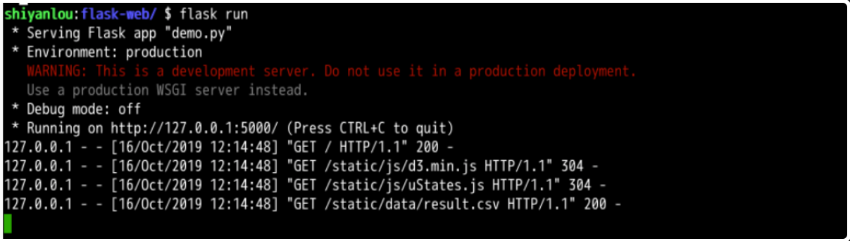
Execute the following command in the flash web directory to start the service:

export FLASK_APP=demo.py
flask run

The results are as follows:

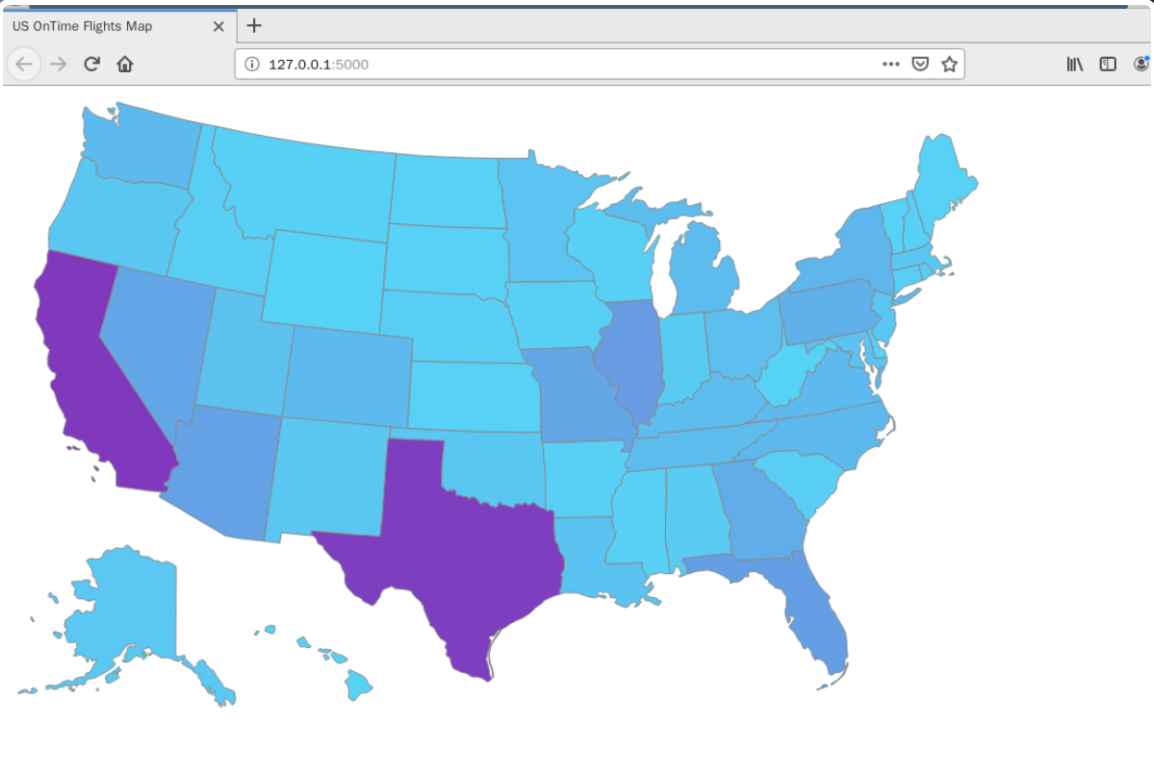
Access address in browser: http://127.0.0.1:5000 A map of the United States. Point to each state with the mouse and you can see the corresponding details.

Do you feel the strong impact of the data?

As you can see, the two states with the deepest colors in the figure are CA and TX. To some extent, it shows that the aviation activities in the two states are more active.

Experimental summary

In this experiment, we analyze the recorded data of flight take-off and landing through Spark based on common DataFrame and SQL operations, find out the causes of flight delay, and predict the flight delay by using machine learning algorithm.

And use D3 JS, the number of on-time flights in American States is visualized. D3 was involved in the experiment JS for reading data, interpolation, selecting elements, setting attributes and other API usage.

If you are interested in analyzing the data of other years, you may find the following interesting phenomena:

• In summer, due to the increase of thunderstorms and other bad weather, flight delays are serious.
• In winter, due to less bad weather and stable climate, flight delays are less.
  /js/d3.min.js">
  
  ...
  d3.csv("/static/data/result.csv", function(error, csvData) {
  ...

stay flask-web Execute the following command under the directory to start the service:

```python
export FLASK_APP=demo.py
flask run

The results are as follows:

[external chain picture transferring... (img-qGhPNje6-1622437121584)]

Access address in browser: http://127.0.0.1:5000 , a picture of the United States was displayed. Point to each state with the mouse and you can see the corresponding details.

[external chain picture transferring... (img-QXYCffVN-1622437121585)]

Do you feel the strong impact of the data?

As you can see, the two states with the deepest colors in the figure are CA and TX. To some extent, it shows that the aviation activities in the two states are more active.

Experimental summary

In this experiment, we analyze the recorded data of flight take-off and landing through Spark based on common DataFrame and SQL operations, find out the causes of flight delay, and predict the flight delay by using machine learning algorithm.

And use D3 JS, the number of on-time flights in American States is visualized. D3 was involved in the experiment JS for reading data, interpolation, selecting elements, setting attributes and other API usage.

If you are interested in analyzing the data of other years, you may find the following interesting phenomena:

• In summer, due to the increase of thunderstorms and other bad weather, flight delays are serious.
• In winter, due to less bad weather and stable climate, flight delays are less.
• After the September 11 terrorist attacks (September 11, 2001), the number of flights decreased sharply. In the 9 / 11 incident, American Airlines and United Airlines lost two planes respectively, and the whole air transportation was suspended for three days. After resuming the flight, due to the shock of the incident, the number of American Airlines passengers contracted sharply in a short time, and even there was only one passenger on a flight.