It's very popular to master xxx in 24 hours. I think 24 hours is too long. It's better to try 2.4 hours.
I will try to explain complex things in simple terms.
Mankind has been exploring the truth of the universe, or the formula of the universe. When King Wen of Zhou made the book of changes, he was nothing more than calculating predictions through various divinatory symbols. To be frank, I'm looking for a formula like y=f(x1,x2,x3,...). Deduce the result y through x1,x2,x3.
Let me define the definition of machine learning. Generally speaking, let the machine deduce the formula of f(x1,x2,x3) through a large number of samples (x1,y1) (x2,y2)... (xn,yn) (commonly known as big data big data). Note that machine learning can only deduce the formula closest to the truth from the sample, but it can't answer why or explain the principle.
Even if you have never been exposed to machine learning, you must know that it is a very complex subject. Obviously, the introduction should start from the simplest. This article won't teach you what API to call. In this way, you will become a package man. Let's start from the simplest principle.
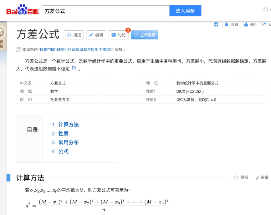
As a folk scientist, first open Baidu Encyclopedia and search "variance formula", you can see the following information:

Here I'll explain Taylor series more popularly. I know that readers of the introductory course will not learn too deep mathematical foundation, so I will only explain it very frankly. To put it bluntly, Taylor just wants to put any y=f(x)The essence of transforming a polynomial into a computable polynomial is to interpret a line of any law into the sum of polynomials. Because one line wants to be equivalent to another line, as long as they are at any time x The derivative of the point is the same, the derivative of the derivative is the same, the derivative of the derivative is the same, the derivative of the derivative is the same.Then they are the same, so we can put any y=f(x)Decompose into a*x^n + b*x^(n-1) + ......+ c*x^(1) + d With such polynomials, the problem can be further simplified.
As an introductory tutorial, we converge the difficulty to the simplest of Polynomials: c*x^(1)，what? You say? d Is it the simplest one? Well, then converge to the second simple term. that is y=ax Such a straight line.

In other words, any complex formula is ultimately composed of several y= θ x or Y= θ x+b composition. Geometrically speaking, this is a direct, so the simplest machine learning is based on linear regression.

dried food:

Suppose we have several y=θx The purpose is to find outθ. Then we should strive for the mostθMake the result of the variance formula of the sample minimum, which is the most stable and most consistent with the truth of the sample. Note that this is important, which is the core methodology throughout machine learning to minimize the value of the cost function.

In order to find out θ， We define a θ Function of: z = J( θ). Therefore, this function should be as follows:

That is, the variance formula. Get the right θ Minimizing z becomes our new goal.
From the direction of convenient understanding of habits, switch to pairs θ Formula. We convert this formula into the customary y = f(x) formula. We can replace X and y with a and b θ Replace with X. Imagine that the new formula should be:

It takes me a lot of effort to format and write the above formula, so next, let the soul painter play.

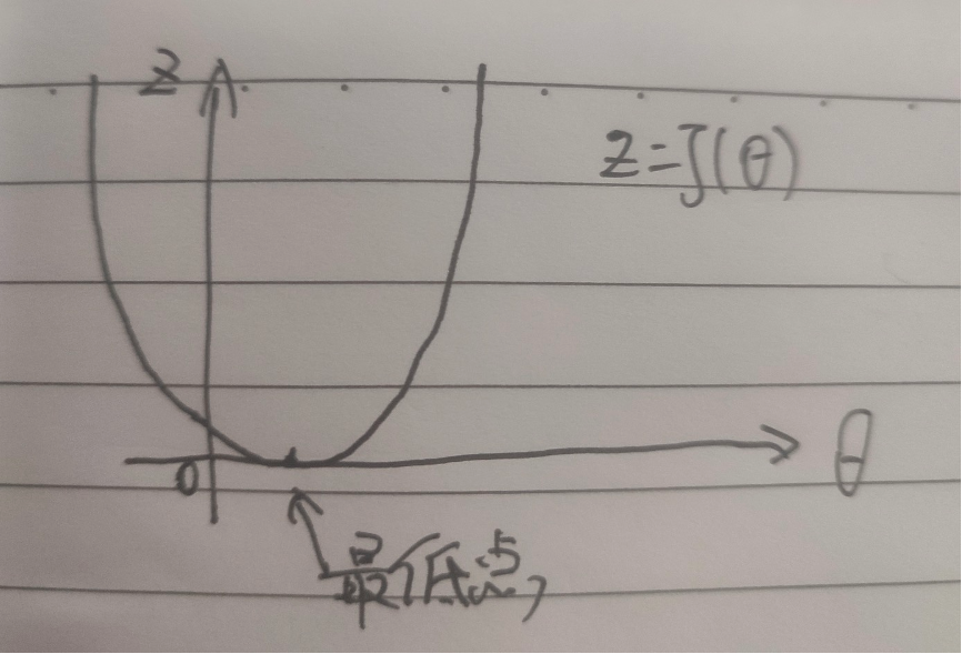
This function is basically J( θ) Well, a U shape (when the variable becomes two-dimensional, you can imagine the shape of a three-dimensional bowl. If it is three-dimensional, it is emo, which I can't imagine), then our purpose is to ask for one θ Value minimizes the value of the curve.
There is a formula that allows θ Gradually approaching the lowest point, this process is called gradient descent method in machine learning. Let's assume that our initial settings θ The value is 0, and then let θ Value becomes θ Value minus an offset until this j( θ) If the derivative of becomes 0, the lowest point is found.

Let's understand from the following figure:

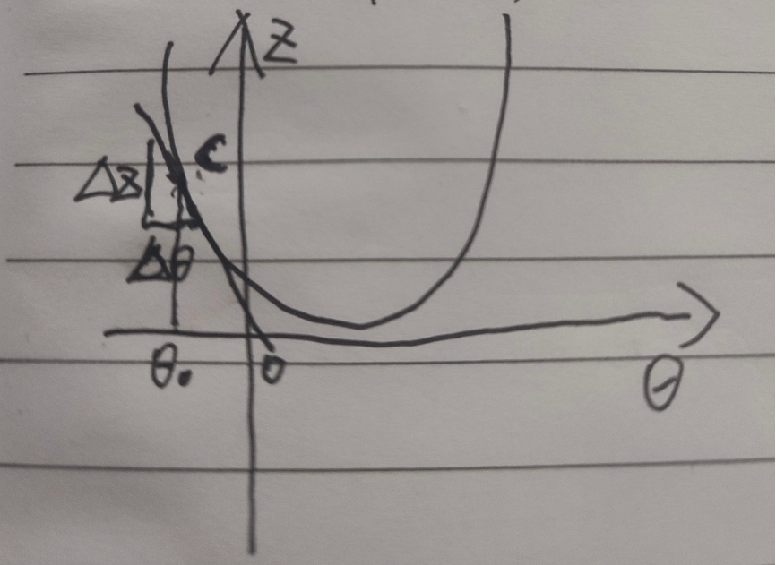
hypothesis θ On the left side of the lowest value, take the derivative of this point, that is, the tangent, and you can get a very small ∆ z and ∆ θ， In fact, their ratio is the derivative of this point, so this is a negative number, soWill let θ Get larger, then move to the right. Similarly, if we take the value on the right, we will let θ Smaller, then move left, when α When it is relatively small, it will gradually approach the lowest point until the derivative is 0 or infinitely close to 0, which is the lowest point.
From above we can seeSo that's

talk is cheap, show you the code.

First, we define the use case of some points

@Data
@NoArgsConstructor
@AllArgsConstructor
public class Case {

    private double x;

    private double y;

    public Case of(double x, double y) {
        return new Case(x, y);
    }
}

We assume that the simplest linear function of y=f(x) is y= θ x. Here θ We set it to a random variable to get the original function

    private static final double REAL_SITA = 12.52D;

    /**
     * Primitive function
     *
     * @param x x value
     * @return y value
     */
    public double orgFunc(double x) {
        return REAL_SITA * x;
    }

Then construct 1000 sample use cases, and assume that the use cases are not very standard, with an error of 5%, which is more realistic

    private static final int CASE_COUNT = 1000;
    private final List<Case> CASES = new ArrayList<>();
    
    /**
     * mock sample
    */
    private void makeCases() {
        List<Case> result = new ArrayList<>();
        for (int i = 0; i < CASE_COUNT; i++) {
            double x = ThreadLocalRandom.current().nextDouble(-100D, 100D);
            double y = orgFunc(x);
            boolean add = ThreadLocalRandom.current().nextBoolean();
            /* For simulation, y perform jitter within 5% */
            int percent = ThreadLocalRandom.current().nextInt(0, 5);
            double f = y * percent / 100;
            if (add) {
                y += f;
            } else {
                y -= f;
            }
            Case c = Case.of(x, y);
            result.add(c);
        }
        /* sort sort */
        result.sort((o1, o2) -> {
            double v = o1.getX() - o2.getX();
            if (v < 0) {
                return -1;
            } else if (v == 0) {
                return 0;
            } else {
                return 1;
            }
        });
        this.CASES.clear();
        this.CASES.addAll(result);
    }

Because we were asked before θ So we can calculate the derivative like this

    /**
     * J(θ)Derivative of
     *
     * @param sita θ
     * @return Derivative value
     */
    public double derivativeOfJ (double sita) {
        double count = 0.0D;
        for (Case c : CASES) {
            double v = sita * c.getX() * c.getX() - c.getX() * c.getY();
            count += v;
        }
        return count / CASE_COUNT;
    }

Finally, we set a smaller one α， Then assume θ The initial value is 0, let θ I keep correcting myself and get the final answer θ value

    /**
     * J(θ)Derivative of
     *
     * @param sita θ
     * @return Derivative value
     */
    public double derivativeOfJ (double sita) {
        double count = 0.0D;
        for (Case c : CASES) {
            double v = sita * c.getX() * c.getX() - c.getX() * c.getY();
            count += v;
        }
        return count / CASE_COUNT;
    }

    /**
     * gradient descent 
     */
    public double stepDownToGetSita() {
        double alpha = 0.0001D;
        /* hypothesis θ Increment from 0 */
        double sita = 0D;
        while (true) {
            double der = derivativeOfJ(sita);
            /* Due to the loss of accuracy of the computer double, when the derivative der infinitely approaches 0, it is considered to be equal to 0 */
            if (Math.abs(der) < 0.000001) {
                return sita;
            }
            /* Or correct it θ */
            sita -= alpha * der;
        }
    }

Finally, we write a junit to test it simply to see if we can calculate the fuzzy value we set in advance θ Values, and real_ What is the specific accuracy of Sita

    @Test
    public void test() {
        LineFunction lineFunction = new LineFunction();
        lineFunction.makeCases();
        double x = lineFunction.stepDownToGetSita();
        log.debug("x:{}", x);
    }

Final output result

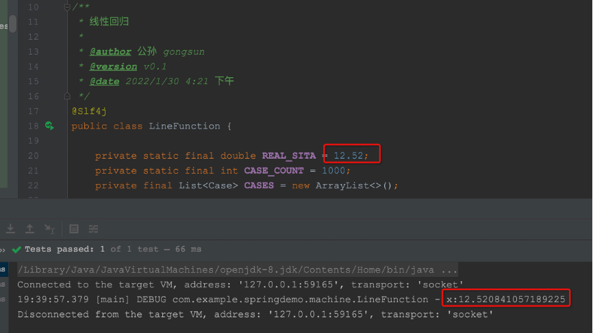
what? You said the result was not very accurate? Well, first, this is just a POC. Second, the number of samples is too small. Third, I fuzzify the samples by 5%, resulting in errors with my own function.
Well, that's the beginning of machine learning. In the future, the complexity of operators will be higher and higher, but that's the principle.