1.VGG16 theory

VGG is a convolutional neural network model proposed by Simonyan and Zisserman in the document very deep revolutionary networks for large scale image recognition. Its name comes from the abbreviation of the visual geometry group of Oxford University where the author works.
The model participated in the ImageNet image classification and positioning challenge in 2014 and achieved excellent results: ranking second in classification tasks and first in positioning tasks. Its structure is shown in the figure below:

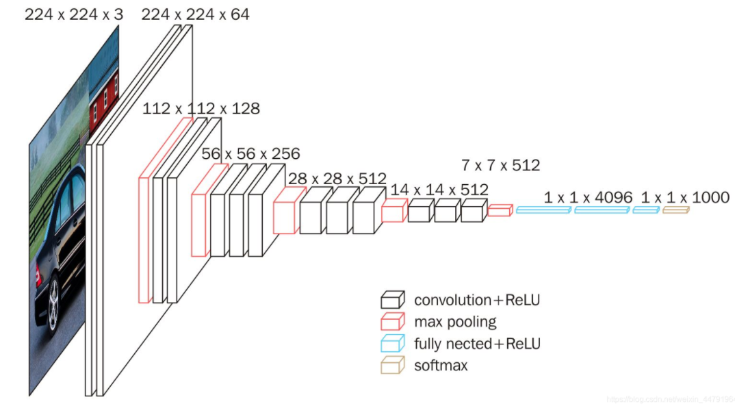
1. An original picture is resize d to (224,3).
2. conv1 twice [3,3] convolution network, the output characteristic layer is 64, the output is (224224,64), and then 2X2 maximizes the pool, and the output net is (112112,64).
3. conv2 twice [3,3] convolution network, the output characteristic layer is 128, the output net is (112112128), and then 2X2 maximum pooling, the output net is (56,56128).
4. conv3 cubic [3,3] convolution network, the output characteristic layer is 256, the output net is (56,56256), and then 2X2 maximizes the pool, and the output net is (28,28256).
5. conv3 cubic [3,3] convolution network, the output characteristic layer is 256, the output net is (28,28512), and then 2X2 maximizes the pool, and the output net is (14,14512).
6. conv3 cubic [3,3] convolution network, the output characteristic layer is 256, the output net is (14,14512), and then 2X2 maximum pooling, the output net is (7,7512).
7. The full connection layer is simulated by convolution, the effect is the same, and the output net is (1,14096). Twice in total.
8. Using convolution to simulate the full connection layer, the effect is the same, and the output net is (1,11000).

in general:

2 convolution layers containing 64 convolution kernels+
2 convolution layers containing 128 convolution kernels+
3 convolution layers containing 256 convolution kernels+
6 convolution layers containing 512 convolution kernels+
Two full junction layers containing 4096 neurons+
1 full junction layer containing 1000 neurons

2. Code implementation

Environment construction: python interpreter: 3.7 + CUDA 10.1 + tensorflow2 three

Data set: we use 11 kinds of motion data collected by ourselves with millimeter wave radar, which are transformed into time-frequency diagram for recognition.

import pathlib
import tensorflow as tf
from tensorflow import keras
from tensorflow.keras import layers,models,Model,Sequential
from tensorflow.keras.layers import Conv2D,BatchNormalization,Activation,Dense,Flatten,MaxPool2D,Dropout
import numpy as np
import matplotlib.pylab as plt

# Prepare data
data_dir = "All_Resize"
data_dir = pathlib.Path(data_dir) # Read out the c1-c10 folder
image_count = len(list(data_dir.glob("*/*")))# The number of images is read out

print("The overview of the picture is:", image_count)

# Parameter setting
batch_size = 4
image_height = 256
image_wijdth = 256

# Partition dataset

train_dst = keras.preprocessing.image_dataset_from_directory(
    data_dir,
    validation_split=None, # Optional floating-point number between 0 and 1. Some data can be reserved for verification
    seed=123, # Optional random seed for shuffle and transformation
    image_size=(image_height, image_wijdth),
    batch_size=batch_size
)

test_dst = keras.preprocessing.image_dataset_from_directory(
    data_dir,
    validation_split=None,
    seed=123,
    image_size=(image_height, image_wijdth),
    batch_size=batch_size
)

# Gets the label of the training set
triain_dst_label = train_dst.class_names
print(triain_dst_label)

AUTOTUME = tf.data.experimental.AUTOTUNE # Dynamically set the number of parallel calls based on the available CPU.
train_dst = train_dst.cache(). shuffle(1000).prefetch(buffer_size=AUTOTUME)
test_dst = test_dst.cache().shuffle(1000).prefetch(buffer_size=AUTOTUME)

# Definition of model
class VGG16(Model):
    def __init__(self):
        super(VGG16, self).__init__()
        # SAME means 0 is filled and VALID means no filling
        """
        2 A convolution layer containing 64 convolution kernels
        """
        self.c1 = Conv2D(filters=64, kernel_size=(3, 3), padding="SAME")
        # Batch standardization prevents the gradient from disappearing, which makes the gradient larger and avoids the problem of gradient disappearing. Moreover, the larger gradient means that the learning convergence speed is fast and the training speed can be greatly accelerated.
        self.b1 = BatchNormalization()
        self.a1 = Activation('relu')
        # 64 convolution kernels
        self.c2 = Conv2D(filters=64, kernel_size=(3, 3), padding="SAME")
        self.b2 = BatchNormalization()
        self.a2 = Activation('relu')
        self.p1 = MaxPool2D(pool_size=(2, 2), strides=2)
        """
        In the machine learning model, if the parameters of the model are too many and the training samples are too few, the trained model is easy to produce the phenomenon of over fitting. When training neural networks
        We often encounter the problem of over fitting, which is manifested in: the loss function of the model in the training data is small, and the prediction accuracy is high; But on the test data, the loss function
        Relatively large, and the prediction accuracy is low.
        Dropout It can effectively alleviate the occurrence of over fitting and achieve the effect of regularization to a certain extent.
        Dropout It can be used as a kind of training depth neural network trick Optional. In each training batch, by ignoring half of the feature detectors (making half of the hidden layer node value 0),
        It can obviously reduce the over fitting phenomenon.
        Dropout To put it simply, when we propagate forward, we make the activation value of a neuron with a certain probability p Stop working, which makes the model more generic because it does not rely too much on some local features
        """
        self.d1 = Dropout(0.2)

        """
        2 A convolution layer containing 128 convolution kernels
        """
        self.c3 = Conv2D(filters=128, kernel_size=(3, 3), padding="SAME")
        self.b3 = BatchNormalization()
        self.a3 = Activation('relu')

        self.c4 = Conv2D(filters=128, kernel_size=(3, 3), padding="SAME")
        self.b4 = BatchNormalization()
        self.a4 = Activation('relu')
        self.p2 = MaxPool2D(pool_size=(2, 2), strides=2)
        self.d2 = Dropout(0.2)

        """
        3 A convolution layer containing 256 convolution kernels
        """
        self.c5 = Conv2D(filters=256, kernel_size=(3, 3), padding="SAME")
        self.b5 = BatchNormalization()
        self.a5 = Activation('relu')

        self.c6 = Conv2D(filters=256, kernel_size=(3, 3), padding="SAME")
        self.b6 = BatchNormalization()
        self.a6 = Activation('relu')

        self.c7 = Conv2D(filters=256, kernel_size=(3, 3), padding="SAME")
        self.b7 = BatchNormalization()
        self.a7 = Activation('relu')
        self.p3 = MaxPool2D(pool_size=(2, 2), strides=2)
        self.d3 = Dropout(0.2)

        """
        6 A convolution layer containing 512 convolution kernels
        """
        self.c8 = Conv2D(filters=512, kernel_size=(3, 3), padding="SAME")
        self.b8 = BatchNormalization()
        self.a8 = Activation('relu')

        self.c9 = Conv2D(filters=512, kernel_size=(3, 3), padding="SAME")
        self.b9 = BatchNormalization()
        self.a9 = Activation('relu')

        self.c10 = Conv2D(filters=512, kernel_size=(3, 3), padding="SAME")
        self.b10 = BatchNormalization()
        self.a10 = Activation('relu')
        self.p4 = MaxPool2D(pool_size=(2, 2), strides=2)
        self.d4 = Dropout(0.2)

        self.c11 = Conv2D(filters=512, kernel_size=(3, 3), padding="SAME")
        self.b11 = BatchNormalization()
        self.a11 = Activation('relu')

        self.c12 = Conv2D(filters=512, kernel_size=(3, 3), padding="SAME")
        self.b12 = BatchNormalization()
        self.a12 = Activation('relu')

        self.c13 = Conv2D(filters=512, kernel_size=(3, 3), padding="SAME")
        self.b13 = BatchNormalization()
        self.a13 = Activation('relu')
        self.p5 = MaxPool2D(pool_size=(2, 2), strides=2)
        self.d5 = Dropout(0.2)

        """
        2 A fully connected layer containing 4096 neurons
        """
        # Flatten layer is used to "flatten" the input, that is, to one dimension the multi-dimensional input, which is often used in the transition from convolution layer to full connection layer. Flatten does not affect the size of the batch.
        self.flatten = Flatten()
        # FC layer is called Dense layer in keras and Linear layer in pytorch
        self.f1 = Dense(4096, activation='relu')
        self.d6 = Dropout(0.2)
        self.f2 = Dense(4096, activation='relu')
        self.d7 = Dropout(0.2)

        """
        1 A fully connected layer containing 11 neurons
        """
        self.f3 = Dense(11, activation='softmax')

    def call(self, x):
         x = self.c1(x)
         x = self.b1(x)
         x = self.a1(x)

         x = self.c2(x)
         x = self.b2(x)
         x = self.a2(x)
         x = self.p1(x)
         x = self.d1(x)

         x = self.c3(x)
         x = self.b3(x)
         x = self.a3(x)

         x = self.c4(x)
         x = self.b4(x)
         x = self.a4(x)
         x = self.p2(x)
         x = self.d2(x)

         x = self.c5(x)
         x = self.b5(x)
         x = self.a5(x)

         x = self.c6(x)
         x = self.b6(x)
         x = self.a6(x)

         x = self.c7(x)
         x = self.b7(x)
         x = self.a7(x)
         x = self.p3(x)
         x = self.d3(x)

         x = self.c8(x)
         x = self.b8(x)
         x = self.a8(x)

         x = self.c9(x)
         x = self.b9(x)
         x = self.a9(x)

         x = self.c10(x)
         x = self.b10(x)
         x = self.a10(x)
         x = self.p4(x)
         x = self.d4(x)

         x = self.c11(x)
         x = self.b11(x)
         x = self.a11(x)

         x = self.c12(x)
         x = self.b12(x)
         x = self.a12(x)

         x = self.c13(x)
         x = self.b13(x)
         x = self.a13(x)
         x = self.p5(x)
         x = self.d5(x)

         x = self.flatten(x)
         x = self.f1(x)
         x = self.d6(x)

         x = self.f2(x)
         x = self.d7(x)

         y = self.f3(x)

         return y

model = VGG16()
opt = tf.keras.optimizers.Adam(learning_rate=1e-4)
"""
model.compile()Method is used to inform the optimizer, loss function and accuracy evaluation standard used in training when configuring the training method
model.compile(optimizer = optimizer, loss = Loss function, metrics = [""Accuracy"])
optimizer It can be the optimizer name given in string form or function form. The learning rate, momentum and super parameters can be set in function form:
            "sgd"  perhaps   tf.optimizers.SGD(lr = Learning rate, decay = Learning rate decay rate, momentum = Momentum parameter)
           "adagrad"  perhaps  tf.keras.optimizers.Adagrad(lr = Learning rate, decay = Learning rate (decay rate)
            "adadelta"  perhaps  tf.keras.optimizers.Adadelta(lr = Learning rate, decay = Learning rate (decay rate)
             "adam"  perhaps  tf.keras.optimizers.Adam(lr = Learning rate, decay = Learning rate (decay rate)
             
loss It can be the name of the loss function given in string form or function form:
           "mse" perhaps tf.keras.losses.MeanSquaredError()
           "sparse_categorical_crossentropy"  perhaps  tf.keras.losses.SparseCatagoricalCrossentropy(from_logits = False)
           The loss function is often used softmax Function to convert the output into the form of probability distribution, here from_logits Represents whether to convert the output to the form of probability distribution, which is False When, it means to convert to probability distribution, and True When, it means no conversion and direct output
Metrics Label network evaluation index:
        "accuracy" : y_ and y All values, such as y_ = [1] y = [1]  #y_ Is the true value and Y is the predicted value
        "sparse_accuracy":y_and y They are expressed in terms of unique heat code and probability distribution, such as y_ = [0, 1, 0], y = [0.256, 0.695, 0.048]
        "sparse_categorical_accuracy" :y_Is given in numerical form, y Is given as a unique heat code, such as y_ = [1], y = [0.256 0.695, 0.048]
"""

model.compile(optimizer=opt, loss=tf.keras.losses.SparseCategoricalCrossentropy(from_logits=False),
              metrics=['sparse_categorical_accuracy'])

history = model.fit(train_dst, validation_data=test_dst, epochs=10)
model.save_weights('VGG16_model.h5')
model.summary()

# View trainable variables
print(model.trainable_variables)

file = open('./weight.txt', 'w')
for v in model.trainable_variables:
    file.write(str(v.name)+'\n')
    file.write(str(v.shape)+'\n')
    file.write(str(v.numpy())+'\n')
file.close()

#############   show    ##################
# Display ACC and Loss of training set and test set
acc = history.history['sparse_categorical_accuracy']
val_acc = history.history['val_sparse_categorical_accuracy']

loss = history.history['loss']
val_loss = history.history['val_loss']

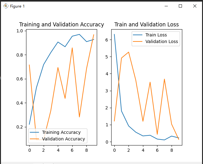
plt.subplot(121)
plt.plot(acc, label='Training Accuracy')
plt.plot(val_acc, label='Validation Accuracy')
plt.title("Training and Validation Accuracy")
plt.legend()

plt.subplot(122)
plt.plot(loss, label='Train Loss')
plt.plot(val_loss, label='Validation Loss')
plt.title("Train and Validation Loss")
plt.legend()
plt.show()

The results are as follows: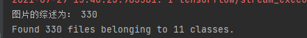

Training process: because our GPU memory is insufficient (mainly afraid to waste my computer), we only iterated for 10 times, so the effect is not good. We tried to iterate for 500 times before, and the effect is 95 You can try if you are interested.