background
The data also have eight characters of birthdays, do you believe it? How do elements and columns, rows and rows interrelate? Is the query slow? Don't believe that everything is destined by heaven. How to change the data? After reading this article, you can do it.
One talent, nine efforts. Fate is destined. The destiny is decided by heaven. It was also said that my fate was beyond my control. It seems that the Chinese ancients had a thorough study of the things congenitally destined, and had a good view of them. However, they also made up for their congenital deficiencies by means of acquired efforts, or by means of transportation reform.

In fact, when I was preparing to write this article, I found that the arrangement of data in the database, the storage of data and the traditional culture related to Chinese numerology are very similar. There are also congenital factors and claims of acquired remedies.
What's the matter? Listen to me carefully.
In order to speed up the efficiency of data retrieval, we usually need to create an index to improve the accuracy of data location. For example, to query someone's monthly call streaming data, without an index, we need to search all the data and match them one by one. By indexing, you can directly locate the records that need to be queried.
Especially when storage and computation are separated, the larger the amount of search, the larger the amount of data transmitted in the network. The bottleneck is obvious.
In addition, in the field of OLAP, a large amount of data needs to be processed. If all the data are indexed, the cost of index introduction is still considerable.
So is there any other way to reduce the amount of scans without indexing?
Storage layer statistics and filtering push-downs
I believe you must have thought that statistics, yes, we can store data by block statistics, such as the data range within each block.
There are several very common technical implementations:
1. PostgreSQL BRIN Index.
https://www.postgresql.org/docs/10/static/brin-intro.html
PostgreSQL brin index is a block-level index, which records the statistics of each block or batch of consecutive blocks.
When searching by this column, irrelevant blocks are filtered through metadata.
2. cstore_fdw column storage plug-in. In fact, it is also stored in columns arranged by BATCH, and the metadata (maximum and minimum) of each BATCH can be used for filtering during scanning.
https://github.com/citusdata/cstore_fdw
Skip indexes: Stores min/max statistics for row groups, and uses them to skip over unrelated rows.
Using Skip Indexes
cstore_fdw partitions each column into multiple blocks. Skip indexes store minimum and maximum values for each of these blocks. While scanning the table, if min/max values of the block contradict the WHERE clause, then the block is completely skipped. This way, the query processes less data and hence finishes faster.
To use skip indexes more efficiently, you should load the data after sorting it on a column that is commonly used in the WHERE clause. This ensures that there is a minimum overlap between blocks and the chance of them being skipped is higher.
In practice, the data generally has an inherent dimension (for example a time field) on which it is naturally sorted. Usually, the queries also have a filter clause on that column (for example you want to query only the last week's data), and hence you don't need to sort the data in such cases.
When searching by this column, irrelevant blocks are filtered through metadata.
Example
Some 300 GB External appearance, sampling skip index Scanning, accelerating scanning.
//It takes 103 milliseconds.

explain (analyze,verbose,timing,costs,buffers) select c400,sum(c2) from ft_tbl1 where c400=1 group by c400;

         Filter: (ft_tbl1.c400 = 1)
         Rows Removed by Filter: 89996
         CStore File: /data01/digoal/pg_root1921/cstore_fdw/13146/41038
         CStore File Size: 325166400400
         Buffers: shared hit=8004
 Planning time: 52.524 ms
 Execution time: 103.555 ms
(13 rows)

//Do not use where c400=1,
//89 seconds
explain (analyze,verbose,timing,costs,buffers) select c400,sum(c2) from ft_tbl1  group by c400;

         CStore File: /data01/digoal/pg_root1921/cstore_fdw/13146/41038
         CStore File Size: 325166400400
         Buffers: shared hit=8004
 Planning time: 52.691 ms
 Execution time: 89428.721 ms
It should be mentioned that the plug-in cstore_fdw does not support parallel computing at present. In fact, the FDW interface of PostgreSQL already supports parallel computing. cstore_fdw can support parallel computing with only a modification.
as follows
https://www.postgresql.org/docs/10/static/fdw-callbacks.html#fdw-callbacks-parallel
Filtration efficiency and linear correlation
Note that not all columns are well filtered because of data storage. For instance:
Writing of a column is very random, resulting in a random distribution of values, so the data range contained in a data block may be relatively large, and the storage element information filtering of this column is very poor.
create table a(id int, c1 int);
insert into a select generate_series(1,1000000), random()*1000000;
The data are distributed as follows
postgres=# select substring(ctid::text, '(\d+),')::int8 blkid, min(c1) min_c1, max(c1) max_c1, min(id) min_id, max(id) max_id from a group by 1 order by 1;
 blkid | min_c1 | max_c1 | min_id | max_id
-------+--------+--------+--------+---------
     0 |   2697 | 998322 |      1 |     909
     1 |   1065 | 998817 |    910 |    1818
     2 |    250 | 998025 |   1819 |    2727
     3 |     62 | 997316 |   2728 |    3636
     4 |   1556 | 998640 |   3637 |    4545
     5 |    999 | 999536 |   4546 |    5454
     6 |   1385 | 999196 |   5455 |    6363
     7 |   1809 | 999042 |   6364 |    7272
     8 |   3044 | 999606 |   7273 |    8181
     9 |   1719 | 999186 |   8182 |    9090
    10 |    618 | 997031 |   9091 |    9999
    11 |     80 | 997581 |  10000 |   10908
    12 |    781 | 997710 |  10909 |   11817
    13 |   1539 | 998857 |  11818 |   12726
    14 |   2097 | 999932 |  12727 |   13635
    15 |    114 | 999913 |  13636 |   14544
    16 |    136 | 999746 |  14545 |   15453
    17 |   2047 | 997439 |  15454 |   16362
    18 |   1955 | 996937 |  16363 |   17271
    19 |   1487 | 999705 |  17272 |   18180
    20 |     97 | 999549 |  18181 |   19089
    21 |    375 | 999161 |  19090 |   19998
    22 |    645 | 994457 |  19999 |   20907
    23 |   4468 | 998612 |  20908 |   21816
    24 |    865 | 996342 |  21817 |   22725
    25 |    402 | 998151 |  22726 |   23634
    26 |    429 | 998823 |  23635 |   24543
    27 |   1305 | 999521 |  24544 |   25452
    28 |    974 | 998874 |  25453 |   26361
    29 |   1056 | 999271 |  26362 |   27270
. . . . . .
For ID columns, the distribution is very clear (with good linear correlation) and the metadata storage is filtered well. The C1 column has very scattered distribution and poor filterability for storing metadata.
For example, I want to look up the data with id=10000, look up block 11 directly, and skip the scanning of other data blocks.
If I want to look up c1=10000 data, I need to look up many data blocks, because there are few data blocks that can be skipped.
How to Improve the Filtration-Storage Arrangement of Each Column
For a single column, the method to improve filtering is very simple, and can be stored in sequence.
For example, in the previous test table, we need to improve the filter performance of C1, which can be achieved by rearranging it according to C1.
After rearrangement, the correlation between C1 column and physical storage (line number) becomes 1 or - 1, that is, linear correlation, so filtering is particularly good.
postgres=# create temp table tmp_a (like a);
CREATE TABLE
postgres=# insert into tmp_a select * from a order by c1;
INSERT 0 1000000
postgres=# truncate a;
TRUNCATE TABLE
postgres=# insert into a select * from tmp_a;
INSERT 0 1000000
postgres=# end;
COMMIT
postgres=# select substring(ctid::text, '(\d+),')::int8 blkid, min(c1) min_c1, max(c1) max_c1, min(id) min_id, max(id) max_id from a group by 1 order by 1;
 blkid | min_c1 | max_c1 | min_id | max_id
-------+--------+--------+--------+---------
     0 |      0 |    923 |   2462 |  999519
     1 |    923 |   1846 |   1487 |  997619
     2 |   1847 |   2739 |    710 |  999912
     3 |   2741 |   3657 |   1930 |  999053
     4 |   3658 |   4577 |   1635 |  999579
     5 |   4577 |   5449 |    852 |  999335
     6 |   5450 |   6410 |    737 |  998277
     7 |   6414 |   7310 |   3262 |  999024
     8 |   7310 |   8245 |    927 |  997907
     9 |   8246 |   9146 |    441 |  999209
    10 |   9146 |  10015 |    617 |  999828
    11 |  10016 |  10920 |   1226 |  998264
    12 |  10923 |  11859 |   1512 |  997404
    13 |  11862 |  12846 |    151 |  998737
    14 |  12847 |  13737 |   1007 |  999250
. . . . . .

c1 Linear correlation between column and physical storage (line number)
postgres=# select correlation from pg_stats where tablename='a' and attname='c1';
 correlation
-------------
           1
(1 row)
Unfortunately, with this arrangement, the filterability of the ID field becomes worse.
Why is that?
Relative linear correlation of two columns in global/full table
In fact, the correlation between ID and C1 columns controls the problem of ID columns becoming discrete after sorting by C1.
What is the correlation between ID and C1?
postgres=# select corr(c1,id) from (select row_number() over(order by c1) c1, row_number() over(order by id) id from a) t;
         corr
-----------------------
 -0.000695987373950136
(1 row)
The poor global (full table) correlation between c1 and id leads to this problem.
(It can be understood that the eight-character inconsistency between the two fields)

Relative linear correlation between two columns of local/partial records
If the whole table is sorted by C1 or ID, the dispersion of the other column becomes very high.
However, in some cases, there may be situations where some records have good correlation between fields A and B, while others have poor correlation.
Example
On the basis of previous records, insert a batch of records.
postgres=# insert into a select id, id*2 from generate_series(1,100000) t(id);
INSERT 0 100000
This part of the data id, the correlation of the C1 field is 1. (Local correlation)
postgres=# select ctid from a offset 1000000 limit 1;
    ctid
------------
 (1113,877)
(1 row)

postgres=# select corr(c1,id) from (select row_number() over(order by c1) c1, row_number() over(order by id) id from a where ctid >'(1113,877)') t;
 corr
------
    1
(1 row)
Global relevance has also improved a lot.
postgres=# select corr(c1,id) from (select row_number() over(order by c1) c1, row_number() over(order by id) id from a) t;
       corr
-------------------
 0.182542794451908
(1 row)
Partial Demand Change Method
Data scattered storage brings problems: even access to a small amount of data will cause a large number of IO reads, the principle is as follows:
Data storage is destined by heaven (it's decided when we write), but we can change our order on demand. For example, one business is the operator's call pipeline, and the query requirement is usually one month's call pipeline based on a certain mobile phone number. In fact, the data is written to the database immediately when it is generated, so the storage is scattered. Query time consumes a lot of IO.
Example
User call data is written in real time, and user data is Brownian distribution.
create table phone_list(phone_from char(11), phone_to char(11), crt_time timestamp, duration interval);
create index idx_phone_list on phone_list(phone_from, crt_time);

insert into phone_list
select
  lpad((random()*1000)::int8::text, 11, '1'),
  lpad((random()*1000)::int8::text, 11, '1'),
  now()+(id||' second')::interval,
  ((random()*1000)::int||' second')::interval
from generate_series(1,10000000) t(id);

postgres=# select * from phone_list limit 10;
 phone_from  |  phone_to   |          crt_time          | duration
-------------+-------------+----------------------------+----------
 14588832692 | 11739044013 | 2017-08-11 10:17:04.752157 | 00:03:25
 15612918106 | 11808103578 | 2017-08-11 10:17:05.752157 | 00:11:33
 14215811756 | 15983559210 | 2017-08-11 10:17:06.752157 | 00:08:05
 13735246090 | 15398474974 | 2017-08-11 10:17:07.752157 | 00:13:18
 19445131039 | 17771201972 | 2017-08-11 10:17:08.752157 | 00:00:10
 11636458384 | 16356298444 | 2017-08-11 10:17:09.752157 | 00:06:30
 15771059012 | 14717265381 | 2017-08-11 10:17:10.752157 | 00:13:45
 19361008150 | 14468133189 | 2017-08-11 10:17:11.752157 | 00:05:58
 13424293799 | 16589177297 | 2017-08-11 10:17:12.752157 | 00:16:29
 12243665890 | 13538149386 | 2017-08-11 10:17:13.752157 | 00:16:03
(10 rows)
Inquiries are inefficient. It takes 26 milliseconds to retrieve 29937 calls from mobile phones.
postgres=# explain (analyze,verbose,timing,costs,buffers) select * from phone_list where phone_from='11111111111' order by crt_time;
                                                                   QUERY PLAN
------------------------------------------------------------------------------------------------------------------------------------------------
 Index Scan using idx_phone_list on public.phone_list  (cost=0.56..31443.03 rows=36667 width=48) (actual time=0.016..24.348 rows=29937 loops=1)
   Output: phone_from, phone_to, crt_time, duration
   Index Cond: (phone_list.phone_from = '11111111111'::bpchar)
   Buffers: shared hit=25843
 Planning time: 0.082 ms
 Execution time: 25.821 ms
(6 rows)
Renovation method, local adjustment on demand.
The requirement is to efficiently query the phone and monthly call details, so we need to rearrange the user's monthly data (usually partitioned monthly).
See the usage of the partition table: PostgreSQL 10.0 preview Enhancement - Built-in Partition Table
postgres=# cluster phone_list using idx_phone_list ;
The efficiency of query has been improved dramatically and the change of order has been successful.
postgres=# explain (analyze,verbose,timing,costs,buffers) select * from phone_list where phone_from='11111111111' order by crt_time;
                                                                  QUERY PLAN
-----------------------------------------------------------------------------------------------------------------------------------------------
 Index Scan using idx_phone_list on public.phone_list  (cost=0.56..31443.03 rows=36667 width=48) (actual time=0.012..4.590 rows=29937 loops=1)
   Output: phone_from, phone_to, crt_time, duration
   Index Cond: (phone_list.phone_from = '11111111111'::bpchar)
   Buffers: shared hit=432
 Planning time: 0.038 ms
 Execution time: 5.968 ms
(6 rows)
You are the hand of God, and the fate of data is in your hands.
How to Improve the Filtration-Storage Arrangement of Each Column
In order to achieve the best filtering performance (each column can be filtered well), global sorting can not meet the requirements.
In fact, you need to sort locally, for example, in the previous example, the first 1 million rows are sorted by C1, and the last 100,000 rows are sorted by ID.
In this way, the ID with 100,000 records is very filterable, and C1 with 1.1 million records is also very filterable.
But numbers are all logical, as if a person's name is also divided into five squares.
Through the remedy acquired, we can change our transportation. Like data arrangement, data rearrangement can affect global filtering and local filtering. Is it interesting?
According to your query target needs, rearrange the data, together to change the transport bar.
Relative Linear Dependence of Multiple Columns in Compound Sorting
How can multiple columns achieve good aggregation for each column?
1. The most sophisticated method, multi-column sorting, but the effect is not necessarily good. In order to achieve better results, we need to adjust the order of columns. The algorithm is as follows:
I remember writing a document like this before:
In fact, it is also the essence of storage arrangement. By arranging and combining, we can calculate the linear correlation of each two columns. According to this, we can find out the best multi-column sorting combination, so as to improve the overall correlation (improve the compression ratio).
The same applies to improving the filterability of all columns mentioned in this article.
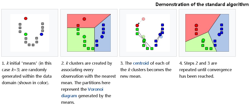
2. k-means algorithm, for multi-column aggregation calculation, completes the best local distribution, so that it can achieve the filtering of each column is very commendable.
K-Means Data Aggregation Algorithms
quintessence
1. Relative correlation between local and global columns. Determines the dispersion of another column after sorting by one column.
2. The purpose of orchestration is to allow as many columns as possible to be stored in an orderly manner so that the most rows can be filtered.
3. Global correlation determines the dispersion of another column when sorted by one column.
4. Local correlation determines the linear correlation of two columns in some records.
5. Arranged by local correlation, more columns can be stored in order as much as possible, so that the most rows can be filtered. However, the algorithm is more complex, which rows need to be calculated together and stored in what order to obtain the best filtering performance.
6. Regarding the arrangement of multi-column (or array) data, method 1 calculates the linear correlation of each two columns (elements) through arrangement and combination, and finds out the best combination of multi-column sorting according to this, so as to improve the overall correlation (increase the compression ratio).
7. After arrangement, if the column with poor linear correlation to storage (line number) has better selectivity (more DISTINCT VALUE) and the service has the need to filter data, it is suggested that index should be built.
8. Regarding the data arrangement of multiple columns (or arrays), method 2 calculates the type of data by kmean, and stores each type aggregately, so as to improve the local aggregation and filtering of data. This method is the most elegant.
9. By choreographing and combining with the BRIN index of PG, the efficient filtering of any column can be realized.
Case Study of Data Renewal
1. Multi-column Change of Order
Low-level methods, A Simple Algorithms Can Help Internet of Things, Financial Users Save 98% of Data Storage Cost (PostgreSQL,Greenplum Help You Do it)
Advanced methods, K-Means Data Aggregation Algorithms
Examples of advanced methods
-- Write 100 million records
-- Heaven's fate, scattered, five elements disorder, inefficient inquiry.
postgres=# create table tab(c1 int, c2 int, c3 int, c4 int, c5 int);
CREATE TABLE
postgres=# insert into tab select * from (select id,100000000-id,50000000-id, sqrt(id*2), sqrt(id) from generate_series(1,100000000) t(id)) t order by random();
INSERT 0 100000000
postgres=# select ctid,* from tab limit 10;
  ctid  |    c1    |    c2    |    c3     |  c4   |  c5
--------+----------+----------+-----------+-------+------
 (0,1)  | 76120710 | 23879290 | -26120710 | 12339 | 8725
 (0,2)  | 98295593 |  1704407 | -48295593 | 14021 | 9914
 (0,3)  | 56133647 | 43866353 |  -6133647 | 10596 | 7492
 (0,4)  |   787639 | 99212361 |  49212361 |  1255 |  887
 (0,5)  | 89844299 | 10155701 | -39844299 | 13405 | 9479
 (0,6)  | 92618459 |  7381541 | -42618459 | 13610 | 9624
 (0,7)  | 93340303 |  6659697 | -43340303 | 13663 | 9661
 (0,8)  | 17164665 | 82835335 |  32835335 |  5859 | 4143
 (0,9)  |  2694394 | 97305606 |  47305606 |  2321 | 1641
 (0,10) | 41736122 | 58263878 |   8263878 |  9136 | 6460
(10 rows)

-- Change your life, press K-MEAN Aggregate and adjust five elements, adopt BRIN Indexing achieves efficient filtering of any column.
-- Keep each column consistent in all directions, for example(a,b) (1,100)(2,101), (100,9)(105,15),If categorized into two categories, in filtering A Field selection is good, filtering B Selectivity is also good for fields.
postgres=# create table tbl1(like tab);
CREATE TABLE

-- Because data is stored in blocks, BRIN The index has the smallest granularity as blocks, so the maximum number of clusters can be the number of blocks in the table. For example, 636943 data blocks can be categorized as 636943.
-- Categorizing more than 636943 is meaningless, and categorizing less is possible, for example BRIN The index stores one meta-information per 10 consecutive data blocks, so we can choose to classify it into 63694 categories.
postgres=# select relpages from pg_class where relname='tab';
 relpages
----------
    636943
(1 row)
postgres=# insert into tbl1 select c1,c2,c3,c4,c5 from (select kmeans(array[c1,c2,c3,c4,c5],63694) over() km, * from tab) t order by km;

-- Create any column BRIN Indexes
create index idx_tab_1 on tab using brin(c1,c2,c3) with (pages_per_range=1);
create index idx_tbl1_1 on tbl1 using brin(c1,c2,c3) with (pages_per_range=1);
Using BRIN index, after changing the data, search any column range, improve efficiency, praise
postgres=# explain (analyze,verbose,timing,costs,buffers) select * from tab where c1 between 1 and 100000;
                                                             QUERY PLAN
-------------------------------------------------------------------------------------------------------------------------------------
 Bitmap Heap Scan on public.tab  (cost=4184.33..906532.40 rows=83439 width=20) (actual time=165.626..1582.402 rows=100000 loops=1)
   Output: c1, c2, c3, c4, c5
   Recheck Cond: ((tab.c1 >= 1) AND (tab.c1 <= 100000))
   Rows Removed by Index Recheck: 14427159
   Heap Blocks: lossy=92530
   Buffers: shared hit=96745
   ->  Bitmap Index Scan on idx_tab_1  (cost=0.00..4163.47 rows=17693671 width=0) (actual time=165.307..165.307 rows=925300 loops=1)
         Index Cond: ((tab.c1 >= 1) AND (tab.c1 <= 100000))
         Buffers: shared hit=4215
 Planning time: 0.088 ms
 Execution time: 1588.852 ms
(11 rows)

postgres=# explain (analyze,verbose,timing,costs,buffers) select * from tbl1 where c1 between 1 and 100000;
                                                            QUERY PLAN
-----------------------------------------------------------------------------------------------------------------------------------
 Bitmap Heap Scan on public.tbl1  (cost=4159.34..111242.78 rows=95550 width=20) (actual time=157.084..169.314 rows=100000 loops=1)
   Output: c1, c2, c3, c4, c5
   Recheck Cond: ((tbl1.c1 >= 1) AND (tbl1.c1 <= 100000))
   Rows Removed by Index Recheck: 9
   Heap Blocks: lossy=637
   Buffers: shared hit=4852
   ->  Bitmap Index Scan on idx_tbl1_1  (cost=0.00..4135.45 rows=95613 width=0) (actual time=157.074..157.074 rows=6370 loops=1)
         Index Cond: ((tbl1.c1 >= 1) AND (tbl1.c1 <= 100000))
         Buffers: shared hit=4215
 Planning time: 0.083 ms
 Execution time: 174.069 ms
(11 rows)

postgres=# explain (analyze,verbose,timing,costs,buffers) select * from tab where c2 between 1 and 100000;
                                                             QUERY PLAN
-------------------------------------------------------------------------------------------------------------------------------------
 Bitmap Heap Scan on public.tab  (cost=4183.50..902041.63 rows=82011 width=20) (actual time=165.901..1636.587 rows=100000 loops=1)
   Output: c1, c2, c3, c4, c5
   Recheck Cond: ((tab.c2 >= 1) AND (tab.c2 <= 100000))
   Rows Removed by Index Recheck: 14446835
   Heap Blocks: lossy=92655
   Buffers: shared hit=96870
   ->  Bitmap Index Scan on idx_tab_1  (cost=0.00..4163.00 rows=17394342 width=0) (actual time=165.574..165.574 rows=926550 loops=1)
         Index Cond: ((tab.c2 >= 1) AND (tab.c2 <= 100000))
         Buffers: shared hit=4215
 Planning time: 0.087 ms
 Execution time: 1643.089 ms
(11 rows)

postgres=# explain (analyze,verbose,timing,costs,buffers) select * from tbl1 where c2 between 1 and 100000;
                                                            QUERY PLAN
-----------------------------------------------------------------------------------------------------------------------------------
 Bitmap Heap Scan on public.tbl1  (cost=4156.97..101777.70 rows=86127 width=20) (actual time=157.245..169.934 rows=100000 loops=1)
   Output: c1, c2, c3, c4, c5
   Recheck Cond: ((tbl1.c2 >= 1) AND (tbl1.c2 <= 100000))
   Rows Removed by Index Recheck: 115
   Heap Blocks: lossy=638
   Buffers: shared hit=4853
   ->  Bitmap Index Scan on idx_tbl1_1  (cost=0.00..4135.44 rows=86193 width=0) (actual time=157.227..157.227 rows=6380 loops=1)
         Index Cond: ((tbl1.c2 >= 1) AND (tbl1.c2 <= 100000))
         Buffers: shared hit=4215
 Planning time: 0.084 ms
 Execution time: 174.692 ms
(11 rows)

postgres=# explain (analyze,verbose,timing,costs,buffers) select * from tab where c3 between 1 and 10000;
                                                             QUERY PLAN
-------------------------------------------------------------------------------------------------------------------------------------
 Bitmap Heap Scan on public.tab  (cost=4141.01..672014.67 rows=9697 width=20) (actual time=191.075..10765.038 rows=10000 loops=1)
   Output: c1, c2, c3, c4, c5
   Recheck Cond: ((tab.c3 >= 1) AND (tab.c3 <= 10000))
   Rows Removed by Index Recheck: 99990000
   Heap Blocks: lossy=636943
   Buffers: shared hit=641158
   ->  Bitmap Index Scan on idx_tab_1  (cost=0.00..4138.58 rows=2062044 width=0) (actual time=190.292..190.292 rows=6369430 loops=1)
         Index Cond: ((tab.c3 >= 1) AND (tab.c3 <= 10000))
         Buffers: shared hit=4215
 Planning time: 0.086 ms
 Execution time: 10766.036 ms
(11 rows)

postgres=# explain (analyze,verbose,timing,costs,buffers) select * from tbl1 where c3 between 1 and 10000;
                                                           QUERY PLAN
---------------------------------------------------------------------------------------------------------------------------------
 Bitmap Heap Scan on public.tbl1  (cost=4137.85..17069.21 rows=10133 width=20) (actual time=150.710..152.040 rows=10000 loops=1)
   Output: c1, c2, c3, c4, c5
   Recheck Cond: ((tbl1.c3 >= 1) AND (tbl1.c3 <= 10000))
   Rows Removed by Index Recheck: 205
   Heap Blocks: lossy=65
   Buffers: shared hit=4280
   ->  Bitmap Index Scan on idx_tbl1_1  (cost=0.00..4135.32 rows=10205 width=0) (actual time=150.692..150.692 rows=650 loops=1)
         Index Cond: ((tbl1.c3 >= 1) AND (tbl1.c3 <= 10000))
         Buffers: shared hit=4215
 Planning time: 0.083 ms
 Execution time: 152.546 ms
(11 rows)
2. Array Renewal
K-Means Data Aggregation Algorithms
3. Spatiotemporal Data Renewal
4. Renewal of Securities System
Related technology
1. Column Storage Plug-in cstore
https://github.com/citusdata/cstore_fdw
https://www.postgresql.org/docs/10/static/fdw-callbacks.html#fdw-callbacks-parallel
https://www.postgresql.org/docs/10/static/brin-intro.html
4. metascan is a database function developed by Aliyun PostgreSQL Kernel Team, which has been used RDS PostgreSQL and HybridDB for PostgreSQL In the future, it can also be integrated into the storage engine level, pushing the FILTER of data down to the storage layer. According to the query conditions provided by users, the scanning amount of data can be reduced and the efficiency can be improved without indexing.
We have tested that query performance has improved by three to five times (compared with no index). Writing performance is at least twice as good as indexing.