perceptron is a linear classification model of two kinds of classification. Its input is feature vector and output is instance classification. It takes two values of "-1" and "+1".
Simply put: the perceptron is a hyperplane, which divides the training data into linear parts. With the help of the trained hyperplane and input test data, the predicted results can be obtained.
Not much to say:
Explain the principle!
Get ready:
Suppose that the input space (feature space) is X < R(n), and the output space is Y={-1,+1}.
X corresponds to X, representing the eigenvector of the instance, corresponding to the point in the input space, and outputting y < Y. There are inputs to outputs, corresponding to the function f(x)=sign(w. x+b) (where W. x means inner product, which is wi*xi)
w is usually called weight, b is called bias and sign is a sign function.
sign(x)={+1, x >= 0; - 1, x < 0}

Perceptron is a linear classification model, which belongs to the discriminant model. The assumption space of the perceptron model is a set of hyperplanes, that is, the set of functions {f|f(x)=w. x+b}.

Why is a set not a hyperplane enough?
Explain this: Perceptrons can generate different hyperplanes because of the different order in which they select test cases, that is, all hyperplanes can be judged independently.

Geometric interpretation of perceptron: linear equation: w. x+b=0

key words:

1. Linear separability of data:
   If there is a hyperplane that can divide the training data set into two sides exactly, the data set is called linear separable data set.
2. The distance from a point x0 in the input space to the hyperplane S is: | W. x0 + B |/| w |, where | w | is the L2 norm of w, i.e. | | w |= [w. w]= (wi*wi)
3. Los - function: For an example of misclassification (xi,yi), it always satisfies - yi*(w. Xi + b) > 0. because
   (1) W. xi+b > 0, Yi = 1; (2) W. xi+b < 0, Yi = + 1, so the total distance from the misclassified point to the hyperplane is - yi(w. xi+b)/| | w |. Without considering | w |, the loss function L(w,b) = - yi(w. xi+b) is obtained. It is easy to see that this is a continuous derivative function of W and b, which is one of the reasons why we choose it as the loss function. The later gradient descends and it will show great prestige.
   On the proof of Noviloff:
   Welcome to Dr.cyr's Knowledge Column
   algorithm: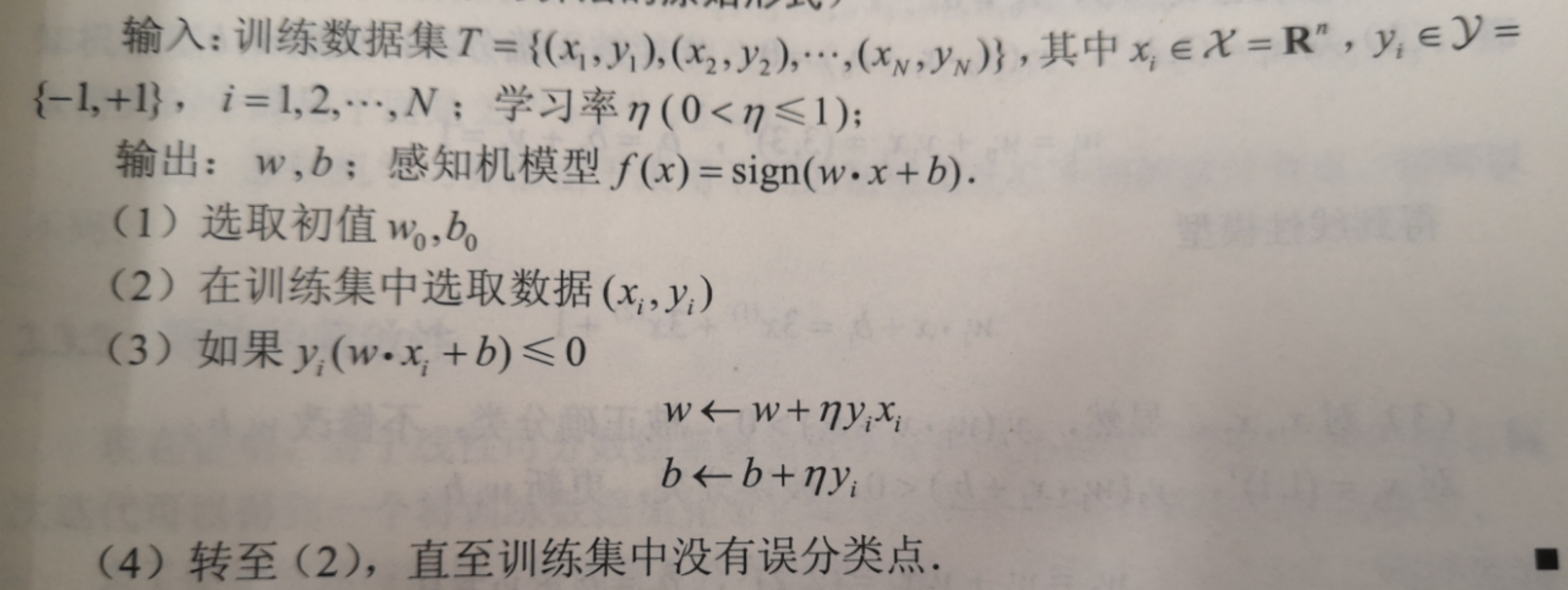
   
   This algorithm is not too difficult to understand, mainly the idea of traversal and iteration.
   Emphasis is placed on updating parameters (w,b):
   Remember the loss function L(w,b) = - yi(w. xi+b), for which we have to de-derive separately.
   ▽w = -∑yixi, ▽b= -∑yi
   Why do you require guidance?
   This method is similar to the random gradient descent method. The purpose of derivation is to continuously reduce the value of loss function and set learning rate, which can be understood as adjustment function. As for learning rate, it can not be set too large, too large will lead to miss the optimal option, too small will lead to too long operation time and easy to fall into local optimum. For novices, the adjustment of learning rate mainly depends on trying.

It's almost the same principle, so let's start with the code implementation.
First, the python initialization version is implemented:

import numpy as np
import matplotlib.pyplot as plt
class MyPerceptron:
    def __init__(self):
        self.w = None
        self.b = 0
        self.l_rate = 1
    def draw(self,x,y,w,b):
        fig = plt.figure()
        ax = fig.add_subplot(111)#Read from left to right, divide the canvas into rows and columns, and draw a picture.
        ax.set_title('perceptron_show')
        plt.xlabel('x(1)')
        plt.ylabel('x(2)')
        #Drawing scatter plots
        for i in range(np.shape(x)[0]):
            if y[i] == -1: #If the counterexample is taken, the dot is drawn with "-"
                ax.scatter(x[i][0],x[i][1],c = 'r',marker = '_')
            else:#If we take the positive example, we use "+" to draw dots.
                ax.scatter(x[i][0],x[i][1],c = 'r',marker = '+')
        #Drawing a hyperplane, the hyperplane in the algorithm: w. x+b=0, so x_2_new can be obtained from x_1_new. Note that this is only a demonstration of two-dimensional hyperplane.
        x1_new = np.arange(0,10,1)
        x2_new = (-b - w[0]*x1_new)/w[1]
        plt.plot(x1_new,x2_new,"b-")
        plt.show()
    #Core Algorithmic Code Invasion
    def fit(self,X_train,y_train):
        self.w = np.zeros(np.shape(X_train)[1])#shape[1] denotes the number of columns
        times = 0
        while times < np.shape(y_train)[0]:#shape[0] denotes the number of rows
            x = X_train[times]
            y = y_train[times]
            if y*(np.dot(self.w,x)+self.b) <= 0:
                self.w = self.w + self.l_rate * np.dot(y,x)
                self.b = self.b + self.l_rate * y
                times = 0
            else:
                times += 1
if __name__=="__main__":
    X_train = [[3,3],[4,3],[1,1]]
    Y_train = [1,1,-1]
    perceptron = MyPerceptron()
    perceptron.fit(X_train,Y_train)
    print(perceptron.w)
    print(perceptron.b)
    perceptron.draw(X_train,Y_train,perceptron.w,perceptron.b)

Here's the sk_learn implementation
It is worth mentioning that the internal parameters of perceptron

1. penalty is a regularization term, and can choose "l1" or "l2", "elastic net". L1 makes features sparser and L2 makes weights more uniform.
2. alpha is a regularization coefficient, too small has no constraint effect, too large has excessive constraint, resulting in under-fitting.
3. eta is the learning rate. In this experiment, because w and b are initially 0, eta will not have any effect on the final result, because the learning rate is always eliminated in the end.
4. max_iter is the maximum number of iterations
5. tol is the termination condition, generally loss reaches a certain range of start-up, when it starts, it can stop iteration.

from sklearn.linear_model import Perceptron
if __name__=="__main__":
    X_train = [[3, 3], [4, 3], [1, 1]]
    Y_train = [1,1,-1]
    #The default values for perceptron internal parameters are as follows
    perceptron = Perceptron(penalty= None,alpha=0.001,eta0=1,max_iter = 5,tol=None)
    #fit function for training
    perceptron.fit(X_train,Y_train)
    #"coef_" refers to the eigenvector, and "intercept_" refers to the bias.
    print("the wight :",perceptron.coef_,"\nbias:",perceptron.intercept_)
    #Accuracy score()
    res = perceptron.score(X_train,Y_train)
    #n_iter is the number of iterations
    print("the n_iter: ",perceptron.n_iter_)
    print("correct rate:{:.0%}".format(res))

Write at the end:
The perceptron has two algorithms, one is the original algorithm, the other is the dual algorithm.
When the training data set N is too large, the original algorithm is chosen, and when the dimension is relatively high, the dual algorithm is chosen, which can reduce the operation cost.
If you have time later, write about the implementation of the dual algorithm (slipped away)