There is nothing to do during the summer vacation, thinking about data mining, this blog is also written in the case of my first study of MATLAB (code can be placed directly in a file).
On the one hand, I want to deepen my understanding, on the other hand, I hope that I can give a reference to the readers who feel unable to start using MATLAB and learning decision tree to understand the processing of each link. By the way, I have used 10 fold cross validation for data sets; of course, my understanding of code is far less than that. There is no magic in directing the direction of the heart and the realm of the code, so the reader should be assured and patiently check (these codes are not long and repetitive). This blog article is just to attract the jade, in order to draw out those pearls and jewels. After all, learning alone without friends is crude and unknown.
Don't talk nonsense, just start. A skillful woman can hardly cook without rice. No matter how skillful she is, she can only stare at her without data. The data we use is the wine data of UCI. The website is as follows: https://archive.ics.uci.edu/ml/datasets/Wine
As for how to process data, please refer to this blog: https://blog.csdn.net/qq_32892383/article/details/82225663#title1
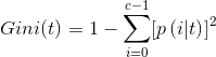
Now that you have learned the decision tree, you must have heard the algorithms ID3 and ID4, and you must know the impurity measures, but here are three entropy measures: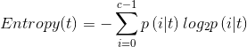

We choose the first measure of information entropy.
- Processing data first
clear
clc
f=fopen('C:\Users\HP\Desktop\Big data\wine.data');
wine=textscan(f,'%f%f%f%f%f%f%f%f%f%f%f%f%f%f','delimiter',',');
fclose(f);
%Put the label in the last column
[m,n]=size(wine);
for i=1:n-1
    data(:,i)=wine{:,i+1};
end
data(:,n)=wine{:,1};
- Our calculation revolves around the calculation of entropy, so we need to write a function to calculate the entropy. This excludes the case of 0*log0=NaN
%%
%The Function of Computing Entropy
function  [Ent_A,Ent_B]=Ent(data,lamda)
%data A data set arranged according to an attribute
%lamda The position of the record after sorting by an attribute
c=3;   %c Act as label Number of Categories
[m,n]=size(data);
data1=data(1:lamda,:);
data2=data(lamda+1:end,:);
Ent_A=0; Ent_B=0;
   %Computational Entropy
for i=1:c
    data1_p(i)=sum(data1(:,n)==i)/lamda;
    if data1_p(i)~=0
        Ent_A=Ent_A-data1_p(i)*log2(data1_p(i));
    end
    data2_p(i)=sum(data2(:,n)==i)/(m-lamda);
    if data2_p(i)~=0
        Ent_B=Ent_B-data2_p(i)*log2(data2_p(i));
    end
end
end
- This is just to calculate the entropy. Then how do we choose the best attribute? So we write a function to find the optimal attribute and return its optimal fraction value, i. e. the threshold value. To maximize the information gain is to minimize the mean entropy. I don't need to calculate the information gain. But here I see an exercise that says that after dividing a node into smaller successor nodes, the node entropy will not increase. (This book is called Introduction to Data Mining, Pang-Ning Tan et al.) I'm not sure about the conclusion that I don't have a proof of mathematical process. I don't want to think about it myself. I want to verify that if Gain < 0 is the calculated information gain, then this conclusion is wrong. Please forgive my laziness.
- I want to say one more thing: because they are continuous values, unlike discrete attributes, using this attribute will not be used, will be used again. Because it's hard for you to ensure that the samples are classified according to an attribute, and no longer classified according to that attribute.
%%
%Searching for optimal sub-attributes attribute
%Optimized Fractional Value value
%Location Division lamda
function [attribute,value,lamda]=pre(data);
total_attribute=13;  %Number of attributes
Ent_parent=0;  %Parent Node Entropy
c=3;
[m,n]=size(data);
for j=1:c
    data_p(j)=sum(data(:,n)==j)/m;
    if data_p(j)~=0
        Ent_parent=Ent_parent-data_p(j)*log2(data_p(j));
    end
end
%Computational optimization sub-attributes
min_Ent=inf;
for i=1:total_attribute
    data=sortrows(data,i);
    for j=1:m-1
        if data(j,n)~=data(j+1,n)
            [Ent_A,Ent_B]=Ent(data,j);
            Ent_pre=Ent_A*j/m+Ent_B*(m-j)/m;
            if Ent_pre<min_Ent
               min_Ent=Ent_pre;
               %Record partition values and attributes at this time
               attribute=i;
               value=data(j,i);
               lamda=j;
            end
        end
    end
    %information gain
    gain=Ent_parent-min_Ent;
    if gain<0
        disp('The algorithm is wrong. Please redesign it.');
        return
    end
end
end
- By finding the optimal sub-attributes, the decision tree classification can be established, and the decision tree can be established recursively. Once you are familiar with recursion, you can be said to be an intermediate level. Here, I choose the accuracy P in the main program is 90%, that is, more than 90% of the samples in a sample are of the same kind, so there is no need to re-establish the judgment conditions.
 - %%
%Establishing Decision Tree
%P Control accuracy to prevent excessive branching, i.e. over-fitting
function tree=decision_tree(data,P)
[m,n]=size(data);
c=3;
tree=struct('value','null','left','null','right','null');
[attribute,value,lamda]=pre(data);
data=sortrows(data,attribute);
tree.value=[attribute,value];
tree.left=data(1:lamda,:);
tree.right=data(lamda+1:end,:);
%Termination of Construction Conditions
for i=1:c
    left_label(i)=sum(tree.left(:,n)==i);
    right_label(i)=sum(tree.right(:,n)==i);
end
    [num,max_label]=max(left_label);
    if num~=lamda&&(num/lamda)<P
        tree.left=decision_tree(tree.left,P);
    else
        tree.left=[max_label num];
    end
    [num,max_label]=max(right_label);
    if num~=(m-lamda)&&(num/(m-lamda))<P
        tree.right=decision_tree(tree.right,P);
    else
        tree.right=[max_label num];
    end
end
- However, although we have got the structure of decision tree, we can not avoid some people's harsh requirements, there are no plans. I think so. After all, the picture is more obvious. So in order to draw this tree, we need to do some preparation. It's just preparation. It's still in the main program. The following procedure refers to this blog:
- https://blog.csdn.net/sinat_31857633/article/details/82693202
%%
%Data visualization, preparation for tree drawing
%nodes For 0
%iter 1, record the number of iterations
%A The node information of the tree graph is recorded, including treeplot Node Sequence
function [A,iter]=print_tree(tree,A,iter,nodes)
A{iter,1}=strcat('attribute:',num2str(tree.value(1)));
A{iter,2}=strcat('threshold:',num2str(tree.value(2)));
A{iter,3}=nodes;
iter=iter+1;nodes=iter-1;
if isstruct(tree.left)
    [A,iter]=print_tree(tree.left,A,iter,nodes);
else
    A{iter,1}=strcat('label:',num2str(tree.left(1)));
    A{iter,2}=strcat('Number:',num2str(tree.left(2)));
    A{iter,3}=nodes;
    iter=iter+1;
end
if  isstruct(tree.right)
    [A,iter]=print_tree(tree.right,A,iter,nodes);
else
    A{iter,1}=strcat('label:',num2str(tree.right(1)));
    A{iter,2}=strcat('Number:',num2str(tree.right(2)));
    A{iter,3}=nodes;
    iter=iter+1;
end
end
- The decision tree and a main program are supposed to be finished here, but as I said earlier, I used 10 fold cross validation for data sets, so I have to write a function of the test tree.
%%
%Calculate the number of correct and error categories in the test set
function [right,error]=testtree(tree,test,right,error)
%right Number of correct categories judged on behalf of the test set
%error Number of error categories judged on behalf of the test set
attribute=tree.value(1);
value=tree.value(2);
test_left=test(find(test(:,attribute)<=value),:);
test_right=test(find(test(:,attribute)>value),:);
if isstruct(tree.left)
    [right,error]=testtree(tree.left,test_left,right,error);
else
    [m,n]=size(test_left);
    for i=1:m
        if test_left(i,n)==tree.left(1)
            right=right+1;
        else
            error=error+1;
        end
    end
end
if isstruct(tree.right)
    [right,error]=testtree(tree.right,test_right,right,error);
else
    [m,n]=size(test_right);
    for i=1:m
        if test_right(i,n)==tree.right(1)
            right=right+1;
        else
            error=error+1;
        end
    end
end
end
Plus the main program:
%%
%main program
%Cross-validation
%10 Sub-10 fold cross-validation partitioning data sets
cov_iter=1;%Number of iterations for cross validation
k=10;%Divide 10 subsets
while cov_iter<=k
train=data;
train_index=0;
test_index=1;
for i=1:3
    s=sum(data(:,n)==i);
    total=round(s/k);
    sel=randperm(s,total);
    test(test_index:test_index+total-1,:)=data(train_index+sel,:);
    train(train_index+sel,:)=[];
    train_index=train_index+s-total;
    test_index=test_index+total;
end
P=0.9;
tree=decision_tree(train,P);
[right,error]=testtree(tree,test,0,0);
accuracy(cov_iter)=right/(right+error);
cov_iter=cov_iter+1;
end
display(strcat('Average accuracy of test set',num2str(mean(accuracy)*100),'%'));


%Drawing Decision Tree Model
A={};%A Description for nodes
iter=1;%iter For the number of iterations
nodes=0;%Sequence of root nodes
[A,~]=print_tree(tree,A,iter,nodes);
[m,n]=size(A);
for i=1:m
    nodes(i)=A{i,n};
    name1{1,i}=A{i,1};
    name2{1,i}=A{i,2};
end
treeplot(nodes);
[x,y]=treelayout(nodes);
for i=1:m
text(x(1,i),y(1,i),{[name1{1,i}];[name2{1,i}]},'VerticalAlignment','bottom','HorizontalAlignment','center')
end
title(strcat('The accuracy of wine decision tree is as follows',num2str(P*100),'%'));
It's over here. Together, our program is (you just need to change the name of the open file where you can run it) below, if you can not even see the operation, I can only say: Ha ha! Attached below are our pictures and results:
clear
clc
f=fopen('C:\Users\HP\Desktop\Big data\wine.data');
wine=textscan(f,'%f%f%f%f%f%f%f%f%f%f%f%f%f%f','delimiter',',');
fclose(f);
%Put the label in the last column
[m,n]=size(wine);
for i=1:n-1
    data(:,i)=wine{:,i+1};
end
data(:,n)=wine{:,1};
%%
%main program
%Cross-validation
%10 Sub-10 fold cross-validation partitioning data sets
cov_iter=1;%Number of iterations for cross validation
k=10;%Divide 10 subsets
while cov_iter<=k
train=data;
train_index=0;
test_index=1;
for i=1:3
    s=sum(data(:,n)==i);
    total=round(s/k);
    sel=randperm(s,total);
    test(test_index:test_index+total-1,:)=data(train_index+sel,:);
    train(train_index+sel,:)=[];
    train_index=train_index+s-total;
    test_index=test_index+total;
end
P=0.9;
tree=decision_tree(train,P);
[right,error]=testtree(tree,test,0,0);
accuracy(cov_iter)=right/(right+error);
cov_iter=cov_iter+1;
end
display(strcat('Average accuracy of test set',num2str(mean(accuracy)*100),'%'));


%Drawing Decision Tree Model
A={};%A Description for nodes
iter=1;%iter For the number of iterations
nodes=0;%Sequence of root nodes
[A,~]=print_tree(tree,A,iter,nodes);
[m,n]=size(A);
for i=1:m
    nodes(i)=A{i,n};
    name1{1,i}=A{i,1};
    name2{1,i}=A{i,2};
end
treeplot(nodes);
[x,y]=treelayout(nodes);
for i=1:m
text(x(1,i),y(1,i),{[name1{1,i}];[name2{1,i}]},'VerticalAlignment','bottom','HorizontalAlignment','center')
end
title(strcat('The accuracy of wine decision tree is as follows',num2str(P*100),'%'));
%%
%The Function of Computing Entropy
function  [Ent_A,Ent_B]=Ent(data,lamda)
%data A data set arranged according to an attribute
%lamda The position of the record after sorting by an attribute
c=3;   %c Act as label Number of Categories
[m,n]=size(data);
data1=data(1:lamda,:);
data2=data(lamda+1:end,:);
Ent_A=0; Ent_B=0;
   %Computational Entropy
for i=1:c
    data1_p(i)=sum(data1(:,n)==i)/lamda;
    if data1_p(i)~=0
        Ent_A=Ent_A-data1_p(i)*log2(data1_p(i));
    end
    data2_p(i)=sum(data2(:,n)==i)/(m-lamda);
    if data2_p(i)~=0
        Ent_B=Ent_B-data2_p(i)*log2(data2_p(i));
    end
end
end
%%
%Searching for optimal sub-attributes attribute
%Optimized Fractional Value value
function [attribute,value,lamda]=pre(data);
total_attribute=13;  %Number of attributes
Ent_parent=0;  %Parent Node Entropy
c=3;
[m,n]=size(data);
for j=1:c
    data_p(j)=sum(data(:,n)==j)/m;
    if data_p(j)~=0
        Ent_parent=Ent_parent-data_p(j)*log2(data_p(j));
    end
end
%Computational optimization sub-attributes
min_Ent=inf;
for i=1:total_attribute
    data=sortrows(data,i);
    for j=1:m-1
        if data(j,n)~=data(j+1,n)
            [Ent_A,Ent_B]=Ent(data,j);
            Ent_pre=Ent_A*j/m+Ent_B*(m-j)/m;
            if Ent_pre<min_Ent
               min_Ent=Ent_pre;
               %Record partition values and attributes at this time
               attribute=i;
               value=data(j,i);
               lamda=j;
            end
        end
    end
    %information gain
    gain=Ent_parent-min_Ent;
    if gain<0
        disp('The algorithm is wrong. Please redesign it.');
        return
    end
end
end
%%
%Establishing Decision Tree
%P Control accuracy to prevent excessive branching, i.e. over-fitting
function tree=decision_tree(data,P)
[m,n]=size(data);
c=3;
tree=struct('value','null','left','null','right','null');
[attribute,value,lamda]=pre(data);
data=sortrows(data,attribute);
tree.value=[attribute,value];
tree.left=data(1:lamda,:);
tree.right=data(lamda+1:end,:);
%Termination of Construction Conditions
for i=1:c
    left_label(i)=sum(tree.left(:,n)==i);
    right_label(i)=sum(tree.right(:,n)==i);
end
    [num,max_label]=max(left_label);
    if num~=lamda&&(num/lamda)<P
        tree.left=decision_tree(tree.left,P);
    else
        tree.left=[max_label num];
    end
    [num,max_label]=max(right_label);
    if num~=(m-lamda)&&(num/(m-lamda))<P
        tree.right=decision_tree(tree.right,P);
    else
        tree.right=[max_label num];
    end
end

%%
%Data visualization, preparation for tree drawing
function [A,iter]=print_tree(tree,A,iter,nodes)
A{iter,1}=strcat('attribute:',num2str(tree.value(1)));
A{iter,2}=strcat('threshold:',num2str(tree.value(2)));
A{iter,3}=nodes;
iter=iter+1;nodes=iter-1;
if isstruct(tree.left)
    [A,iter]=print_tree(tree.left,A,iter,nodes);
else
    A{iter,1}=strcat('label:',num2str(tree.left(1)));
    A{iter,2}=strcat('Number:',num2str(tree.left(2)));
    A{iter,3}=nodes;
    iter=iter+1;
end
if  isstruct(tree.right)
    [A,iter]=print_tree(tree.right,A,iter,nodes);
else
    A{iter,1}=strcat('label:',num2str(tree.right(1)));
    A{iter,2}=strcat('Number:',num2str(tree.right(2)));
    A{iter,3}=nodes;
    iter=iter+1;
end
end

%%
%Calculate the number of correct and error categories in the test set
function [right,error]=testtree(tree,test,right,error)
%right Number of correct categories judged on behalf of the test set
%error Number of error categories judged on behalf of the test set
attribute=tree.value(1);
value=tree.value(2);
test_left=test(find(test(:,attribute)<=value),:);
test_right=test(find(test(:,attribute)>value),:);
if isstruct(tree.left)
    [right,error]=testtree(tree.left,test_left,right,error);
else
    [m,n]=size(test_left);
    for i=1:m
        if test_left(i,n)==tree.left(1)
            right=right+1;
        else
            error=error+1;
        end
    end
end
if isstruct(tree.right)
    [right,error]=testtree(tree.right,test_right,right,error);
else
    [m,n]=size(test_right);
    for i=1:m
        if test_right(i,n)==tree.right(1)
            right=right+1;
        else
            error=error+1;
        end
    end
end
end
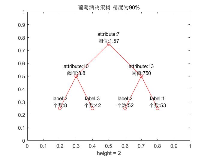
The average accuracy of test set is 95.5556%.