[Wu Enda Machine Learning Assignment 2] - Logical Regression Chapter Python Implementation
Recommended running environment: python 3.6
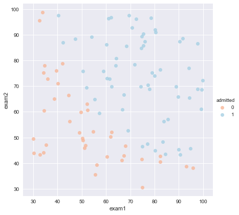
Establish a logistic regression model to predict whether a student will be admitted to a university or not. The admission opportunities of each applicant are determined according to the results of the two examinations. There are historical data of previous applicants.
It can be used as a training set of logistic regression
Training Data Network Disk Link: Link: https://pan.baidu.com/s/1w5r8kMrG4H_J2H9zMDyjVg Extraction Code: 67ec
python realizes logical regression
Objectives: To establish a classifier (to solve three parameters theta 0 theta 1 theta 2) that is, to draw a demarcation line.
Note: Theta 1 corresponds to'Exam 1'and theta 2 corresponds to'Exam 2'.
Setting threshold and judging admission result according to threshold
Note: Threshold refers to the final probability value. Converting the probability value into a category. Generally speaking, more than 0.5 is accepted and less than 0.5 is not accepted.
Realization content:
sigmoid: a function mapped to probability
model: Returns the predicted result value
cost: Calculate losses based on parameters
Gradient: Calculate the gradient direction of each parameter
descent: Update parameters
accuracy: Computational accuracy
import pandas as pd
import numpy as np
import matplotlib.pyplot as plt
import seaborn as sns
plt.style.use('fivethirtyeight') #Style Beautification
import matplotlib.pyplot as plt
from sklearn.metrics import classification_report#This package is an evaluation report.
Preparing data
data = pd.read_csv('ex2data1.txt', names=['exam1', 'exam2', 'admitted'])
data.head()#Look at the first five elements
| exam1 | exam2 | admitted | |
|---|---|---|---|
| 0 | 34.623660 | 78.024693 | 0 |
| 1 | 30.286711 | 43.894998 | 0 |
| 2 | 35.847409 | 72.902198 | 0 |
| 3 | 60.182599 | 86.308552 | 1 |
| 4 | 79.032736 | 75.344376 | 1 |
data.describe()
| exam1 | exam2 | admitted | |
|---|---|---|---|
| count | 100.000000 | 100.000000 | 100.000000 |
| mean | 65.644274 | 66.221998 | 0.600000 |
| std | 19.458222 | 18.582783 | 0.492366 |
| min | 30.058822 | 30.603263 | 0.000000 |
| 25% | 50.919511 | 48.179205 | 0.000000 |
| 50% | 67.032988 | 67.682381 | 1.000000 |
| 75% | 80.212529 | 79.360605 | 1.000000 |
| max | 99.827858 | 98.869436 | 1.000000 |
##Error case1 TypeError:unhashable type :_ColorPalette
Running Problem Replacement Scheme sns.set(context= "notebook", "style="darkgrid","palette=sns.color_palette("RdBu", 2),color_codes=False) because the color of the drawing board is customized
sns.set(context="notebook", style="darkgrid", palette=sns.color_palette("RdBu", 2)) #Set style parameters, default theme darkgrid (grey background + white grid), palette 2 colors

sns.lmplot('exam1', 'exam2', hue='admitted', data=data,
           size=6,
           fit_reg=False,                         #fit_reg'parameter, which controls whether the fitting line is displayed or not
           scatter_kws={"s": 50}
          )                                       #The hue parameter is to superimpose the different types of data specified by name on a graph to display
plt.show()#Look at the data.
def get_X(df):#Read feature
#     """
#     use concat to add intersect feature to avoid side effect
#     not efficient for big dataset though
#     """
    ones = pd.DataFrame({'ones': np.ones(len(df))})#One is the data frame of column 1 of m row
    data = pd.concat([ones, df], axis=1)  # Merge data. When axis = 1 is merged by column, concat is row alignment, and then merge two tables with different column names.
    return data.iloc[:, :-1].as_matrix()  # This operation returns ndarray, not a matrix


def get_y(df):#Read labels
#     '''assume the last column is the target'''
    return np.array(df.iloc[:, -1])#df.iloc[:, -1] is the last column of df


def normalize_feature(df):
#     """Applies function along input axis(default 0) of DataFrame."""
    return df.apply(lambda column: (column - column.mean()) / column.std())#The same applies to feature scaling in logistic regression
X = get_X(data)
print(X.shape)

y = get_y(data)
print(y.shape)
(100, 3)
(100,)
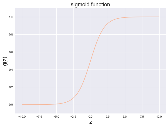
sigmoid function
G stands for a commonly used logic function, which is a S-shaped function. The formula is [g left ( z right)= frac {1} {1+{{e} ^ {z}} ]
Together, we obtain the hypothetical functions of the logistic regression model:
\[{{h}_{\theta }}\left( x \right)=\frac{1}{1+{{e}^{-{{\theta }^{T}}X}}}\]
def sigmoid(z):
    # your code here  (appro ~ 1 lines)
    return 1 / (1 + np.exp(-z))
The following program will call the function you wrote above and draw the sigmoid function image. If your program is correct, you should be able to see the function image below.
fig, ax = plt.subplots(figsize=(8, 6))
ax.plot(np.arange(-10, 10, step=0.01),
        sigmoid(np.arange(-10, 10, step=0.01)))
ax.set_ylim((-0.1,1.1))     #lim axis display length
ax.set_xlabel('z', fontsize=18)
ax.set_ylabel('g(z)', fontsize=18)
ax.set_title('sigmoid function', fontsize=18)
plt.show()
Cost function
- max(ℓ(θ))=min(−ℓ(θ))max(\ell(\theta)) = min(-\ell(\theta))max(ℓ(θ))=min(−ℓ(θ))
- choose −ℓ(θ)-\ell(\theta)−ℓ(θ) as the cost function
KaTeX parse error: No such environment: align at position 7: \begin{̲a̲l̲i̲g̲n̲}̲ & J\left( \t...
theta = theta=np.zeros(3) # X(m*n) so theta is n*1
theta
array([ 0., 0., 0.])
def cost(theta, X, y):
    ''' cost fn is -l(theta) for you to minimize'''
    # your code here  (appro ~ 2 lines)
    return np.mean(-y * np.log(sigmoid(X @ theta)) - (1 - y) * np.log(1 - sigmoid(X @ theta)))
# Hint:X @ theta is equivalent to X.dot(theta)
cost(theta, X, y)
0.69314718055994529
## Error case 269.31 solution y = data. iloc [:, -1]. values y = y. reshape (len (y), 1) example [1,1]
If you write the correct code, the output here should be 0.6931471805599453
Gradient descent
- This is batch gradient descent.
- Conversion to vectorization: 1m XT(Sigmoid(X theta)y)frac {1} {m} X ^ T (Sigmoid (X theta) - y) M1 XT (Sigmoid (Xtheta)y)
∂J(θ)∂θj=1m∑i=1m(hθ(x(i))−y(i))xj(i)\frac{\partial J\left( \theta \right)}{\partial {{\theta }_{j}}}=\frac{1}{m}\sum\limits_{i=1}^{m}{({{h}_{\theta }}\left( {{x}^{(i)}} \right)-{{y}^{(i)}})x_{_{j}}^{(i)}}∂θj∂J(θ)=m1i=1∑m(hθ(x(i))−y(i))xj(i)
def gradient(theta, X, y):
    # your code here  (appro ~ 2 lines)
    return (1 / len(X)) * X.T @ (sigmoid(X @ theta) - y)
gradient(theta, X, y)
array([ -0.1 , -12.00921659, -11.26284221])
Fitting parameters
- Here I use scipy.optimize.minimize To find parameters
import scipy.optimize as opt
res = opt.minimize(fun=cost, x0=theta, args=(X, y), method='Newton-CG', jac=gradient)
## Error case 3 warning: Desired error not necessarily achieved due to precision loss error is mostly cost function problem
## Error case 4 The true value of an array with more than one element is ambiguous. Use A.any () or A.all () Numpy does not distinguish logical expressions clearly. Any means that as long as one True is returned to True,all means that all elements are True will return to True, otherwise False will be returned.
print(res)
     fun: 0.20349770451259855
     jac: array([  1.62947970e-05,   1.11339134e-03,   1.07609314e-03])
 message: 'Optimization terminated successfully.'
    nfev: 71
    nhev: 0
     nit: 28
    njev: 242
  status: 0
 success: True
       x: array([-25.16576744,   0.20626712,   0.20150754])
Prediction and Verification with Training Sets
def predict(x, theta):
    # your code here  (appro ~ 2 lines)
    prob = sigmoid(x @ theta)
    return (prob >= 0.5).astype(int)   #Implementing Variable Type Conversion
final_theta = res.x
y_pred = predict(X, final_theta)

print(classification_report(y, y_pred))
              precision    recall  f1-score   support

           0       0.87      0.85      0.86        40
           1       0.90      0.92      0.91        60

   micro avg       0.89      0.89      0.89       100
   macro avg       0.89      0.88      0.88       100
weighted avg       0.89      0.89      0.89       100
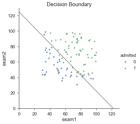
Finding Decision Boundaries
http://stats.stackexchange.com/questions/93569/why-is-logistic-regression-a-linear-classifier
X×θ=0X \times \theta = 0X×θ=0 (this is the line)
print(res.x) # this is final theta
[-25.16576744 0.20626712 0.20150754]
coef = -(res.x / res.x[2])  # find the equation
print(coef)

x = np.arange(130, step=0.1)
y = coef[0] + coef[1]*x
[ 124.88747248 -1.02361985 -1. ]
data.describe() # find the range of x and y
| exam1 | exam2 | admitted | |
|---|---|---|---|
| count | 100.000000 | 100.000000 | 100.000000 |
| mean | 65.644274 | 66.221998 | 0.600000 |
| std | 19.458222 | 18.582783 | 0.492366 |
| min | 30.058822 | 30.603263 | 0.000000 |
| 25% | 50.919511 | 48.179205 | 0.000000 |
| 50% | 67.032988 | 67.682381 | 1.000000 |
| 75% | 80.212529 | 79.360605 | 1.000000 |
| max | 99.827858 | 98.869436 | 1.000000 |
sns.set(context="notebook", style="ticks", font_scale=1.5)  Default use notebook Context Theme context You can set the size of the output picture.(scale)

sns.lmplot('exam1', 'exam2', hue='admitted', data=data,
           size=6,
           fit_reg=False,
           scatter_kws={"s": 25}
          )

plt.plot(x, y, 'grey')
plt.xlim(0, 130)
plt.ylim(0, 130)
plt.title('Decision Boundary')
plt.show()
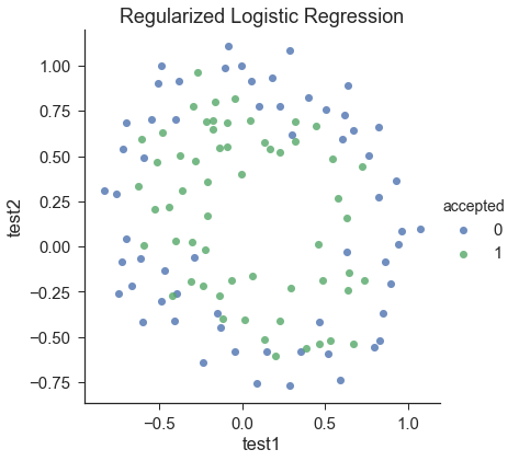
3-Regularized Logical Regression
df = pd.read_csv('ex2data2.txt', names=['test1', 'test2', 'accepted'])
df.head()
| test1 | test2 | accepted | |
|---|---|---|---|
| 0 | 0.051267 | 0.69956 | 1 |
| 1 | -0.092742 | 0.68494 | 1 |
| 2 | -0.213710 | 0.69225 | 1 |
| 3 | -0.375000 | 0.50219 | 1 |
| 4 | -0.513250 | 0.46564 | 1 |
sns.set(context="notebook", style="ticks", font_scale=1.5)

sns.lmplot('test1', 'test2', hue='accepted', data=df,
           size=6,
           fit_reg=False,
           scatter_kws={"s": 50}
          )

plt.title('Regularized Logistic Regression')
plt.show()
feature mapping
polynomial expansion
for i in 0..i
for p in 0..i:
output x^(i-p) * y^p
```
```python
def feature_mapping(x, y, power, as_ndarray=False):
# """return mapped features as ndarray or dataframe"""
data = {"f{}{}".format(i - p, p): np.power(x, i - p) * np.power(y, p)
for i in np.arange(power + 1)
for p in np.arange(i + 1)
}
if as_ndarray:
return pd.DataFrame(data).as_matrix()
else:
return pd.DataFrame(data)
x1 = np.array(df.test1)
x2 = np.array(df.test2)
data = feature_mapping(x1, x2, power=6)
print(data.shape)
data.head()
(118, 28)
| f00 | f01 | f02 | f03 | f04 | f05 | f06 | f10 | f11 | f12 | ... | f30 | f31 | f32 | f33 | f40 | f41 | f42 | f50 | f51 | f60 | |
|---|---|---|---|---|---|---|---|---|---|---|---|---|---|---|---|---|---|---|---|---|---|
| 0 | 1.0 | 0.69956 | 0.489384 | 0.342354 | 0.239497 | 0.167542 | 0.117206 | 0.051267 | 0.035864 | 0.025089 | ... | 0.000135 | 0.000094 | 0.000066 | 0.000046 | 0.000007 | 0.000005 | 0.000003 | 3.541519e-07 | 2.477505e-07 | 1.815630e-08 |
| 1 | 1.0 | 0.68494 | 0.469143 | 0.321335 | 0.220095 | 0.150752 | 0.103256 | -0.092742 | -0.063523 | -0.043509 | ... | -0.000798 | -0.000546 | -0.000374 | -0.000256 | 0.000074 | 0.000051 | 0.000035 | -6.860919e-06 | -4.699318e-06 | 6.362953e-07 |
| 2 | 1.0 | 0.69225 | 0.479210 | 0.331733 | 0.229642 | 0.158970 | 0.110047 | -0.213710 | -0.147941 | -0.102412 | ... | -0.009761 | -0.006757 | -0.004677 | -0.003238 | 0.002086 | 0.001444 | 0.001000 | -4.457837e-04 | -3.085938e-04 | 9.526844e-05 |
| 3 | 1.0 | 0.50219 | 0.252195 | 0.126650 | 0.063602 | 0.031940 | 0.016040 | -0.375000 | -0.188321 | -0.094573 | ... | -0.052734 | -0.026483 | -0.013299 | -0.006679 | 0.019775 | 0.009931 | 0.004987 | -7.415771e-03 | -3.724126e-03 | 2.780914e-03 |
| 4 | 1.0 | 0.46564 | 0.216821 | 0.100960 | 0.047011 | 0.021890 | 0.010193 | -0.513250 | -0.238990 | -0.111283 | ... | -0.135203 | -0.062956 | -0.029315 | -0.013650 | 0.069393 | 0.032312 | 0.015046 | -3.561597e-02 | -1.658422e-02 | 1.827990e-02 |
5 rows × 28 columns
data.describe()
| f00 | f01 | f02 | f03 | f04 | f05 | f06 | f10 | f11 | f12 | ... | f30 | f31 | f32 | f33 | f40 | f41 | f42 | f50 | f51 | f60 | |
|---|---|---|---|---|---|---|---|---|---|---|---|---|---|---|---|---|---|---|---|---|---|
| count | 118.0 | 118.000000 | 118.000000 | 118.000000 | 1.180000e+02 | 118.000000 | 1.180000e+02 | 118.000000 | 118.000000 | 118.000000 | ... | 1.180000e+02 | 118.000000 | 1.180000e+02 | 118.000000 | 1.180000e+02 | 118.000000 | 1.180000e+02 | 1.180000e+02 | 118.000000 | 1.180000e+02 |
| mean | 1.0 | 0.183102 | 0.301370 | 0.142350 | 1.710985e-01 | 0.115710 | 1.257256e-01 | 0.054779 | -0.025472 | 0.015483 | ... | 5.983333e-02 | -0.005251 | 9.432094e-03 | -0.001705 | 1.225384e-01 | 0.011812 | 1.893340e-02 | 5.196507e-02 | -0.000703 | 7.837118e-02 |
| std | 0.0 | 0.519743 | 0.284536 | 0.326134 | 2.815658e-01 | 0.299092 | 2.964416e-01 | 0.496654 | 0.224075 | 0.150143 | ... | 2.746459e-01 | 0.096738 | 5.455787e-02 | 0.037443 | 2.092709e-01 | 0.072274 | 3.430092e-02 | 2.148098e-01 | 0.058271 | 1.938621e-01 |
| min | 1.0 | -0.769740 | 0.000026 | -0.456071 | 6.855856e-10 | -0.270222 | 1.795116e-14 | -0.830070 | -0.484096 | -0.483743 | ... | -5.719317e-01 | -0.296854 | -1.592528e-01 | -0.113448 | 1.612020e-09 | -0.246068 | 2.577297e-10 | -3.940702e-01 | -0.203971 | 6.472253e-14 |
| 25% | 1.0 | -0.254385 | 0.061086 | -0.016492 | 3.741593e-03 | -0.001072 | 2.298277e-04 | -0.372120 | -0.178209 | -0.042980 | ... | -5.155632e-02 | -0.029360 | -3.659760e-03 | -0.005749 | 1.869975e-03 | -0.001926 | 1.258285e-04 | -7.147973e-03 | -0.006381 | 8.086369e-05 |
| 50% | 1.0 | 0.213455 | 0.252195 | 0.009734 | 6.360222e-02 | 0.000444 | 1.604015e-02 | -0.006336 | -0.016521 | -0.000039 | ... | -2.544062e-07 | -0.000512 | -1.473547e-07 | -0.000005 | 2.736163e-02 | 0.000205 | 3.387050e-03 | -1.021440e-11 | -0.000004 | 4.527344e-03 |
| 75% | 1.0 | 0.646562 | 0.464189 | 0.270310 | 2.155453e-01 | 0.113020 | 1.001215e-01 | 0.478970 | 0.100795 | 0.079510 | ... | 1.099616e-01 | 0.015050 | 1.370560e-02 | 0.001024 | 1.520801e-01 | 0.019183 | 2.090875e-02 | 2.526861e-02 | 0.002104 | 5.932959e-02 |
| max | 1.0 | 1.108900 | 1.229659 | 1.363569 | 1.512062e+00 | 1.676725 | 1.859321e+00 | 1.070900 | 0.568307 | 0.505577 | ... | 1.228137e+00 | 0.369805 | 2.451845e-01 | 0.183548 | 1.315212e+00 | 0.304409 | 2.018260e-01 | 1.408460e+00 | 0.250577 | 1.508320e+00 |
8 rows × 28 columns
Regulated cost
J(θ)=1m∑i=1m[−y(i)log(hθ(x(i)))−(1−y(i))log(1−hθ(x(i)))]+λ2m∑j=1nθj2J\left( \theta \right)=\frac{1}{m}\sum\limits_{i=1}^{m}{[-{{y}^{(i)}}\log \left( {{h}_{\theta }}\left( {{x}^{(i)}} \right) \right)-\left( 1-{{y}^{(i)}} \right)\log \left( 1-{{h}_{\theta }}\left( {{x}^{(i)}} \right) \right)]}+\frac{\lambda }{2m}\sum\limits_{j=1}^{n}{\theta _{j}^{2}}J(θ)=m1i=1∑m[−y(i)log(hθ(x(i)))−(1−y(i))log(1−hθ(x(i)))]+2mλj=1∑nθj2
theta = np.zeros(data.shape[1])
X = feature_mapping(x1, x2, power=6, as_ndarray=True)
print(X.shape)

y = get_y(df)
print(y.shape)
(118, 28)
(118,)
def regularized_cost(theta, X, y, l=1):
    # your code here  (appro ~ 3 lines
    theta_j1_to_n = theta[1:]
    regularized_term = (l / (2 * len(X))) * np.power(theta_j1_to_n, 2).sum()

    return  cost(theta, X, y) + regularized_term
regularized_cost(theta, X, y, l=1)
0.6931471805599454
Because we set theta to zero, the regularized cost function should have the same value as the cost function.
Regulated gradient
∂J(θ)∂θj=(1m∑i=1m(hθ(x(i))−y(i)))+λmθj for j≥1\frac{\partial J\left( \theta \right)}{\partial {{\theta }_{j}}}=\left( \frac{1}{m}\sum\limits_{i=1}^{m}{\left( {{h}_{\theta }}\left( {{x}^{\left( i \right)}} \right)-{{y}^{\left( i \right)}} \right)} \right)+\frac{\lambda }{m}{{\theta }_{j}}\text{ }\text{ for j}\ge \text{1}∂θj∂J(θ)=(m1i=1∑m(hθ(x(i))−y(i)))+mλθj for j≥1
def regularized_gradient(theta, X, y, l=1):
    # your code here  (appro ~ 3 lines)
    theta_j1_to_n = theta[1:]      #No theta 0
    regularized_theta = (l / len(X)) * theta_j1_to_n

    regularized_term = np.concatenate([np.array([0]), regularized_theta])
    return gradient(theta, X, y) + regularized_term
regularized_gradient(theta, X, y)
array([  8.47457627e-03,   7.77711864e-05,   3.76648474e-02,
         2.34764889e-02,   3.93028171e-02,   3.10079849e-02,
         3.87936363e-02,   1.87880932e-02,   1.15013308e-02,
         8.19244468e-03,   3.09593720e-03,   4.47629067e-03,
         1.37646175e-03,   5.03446395e-02,   7.32393391e-03,
         1.28600503e-02,   5.83822078e-03,   7.26504316e-03,
         1.83559872e-02,   2.23923907e-03,   3.38643902e-03,
         4.08503006e-04,   3.93486234e-02,   4.32983232e-03,
         6.31570797e-03,   1.99707467e-02,   1.09740238e-03,
         3.10312442e-02])
Fitting parameters
import scipy.optimize as opt
print('init cost = {}'.format(regularized_cost(theta, X, y)))

res = opt.minimize(fun=regularized_cost, x0=theta, args=(X, y), method='Newton-CG', jac=regularized_gradient)
res
init cost = 0.6931471805599454


     fun: 0.5290027297127846
     jac: array([ -1.21895855e-07,   6.76917339e-08,  -2.48482252e-08,
         1.91138610e-08,  -2.53407958e-08,  -1.49952031e-08,
        -1.96092249e-08,   6.15930450e-09,   1.63894777e-08,
         1.46785479e-08,   1.33205342e-08,   8.41414001e-09,
         5.13850532e-09,  -2.89545939e-08,   2.62474472e-08,
        -3.46392476e-08,  -1.57940013e-09,  -1.28923829e-08,
         1.31222180e-08,  -9.17113615e-10,  -1.00687818e-08,
        -3.89939722e-09,  -3.51985068e-08,   1.79476715e-08,
        -1.62131622e-08,   5.09965938e-09,   2.83437559e-09,
        -2.64933033e-08])
 message: 'Optimization terminated successfully.'
    nfev: 7
    nhev: 0
     nit: 6
    njev: 66
  status: 0
 success: True
       x: array([ 1.2727397 ,  1.18108864, -1.43166408, -0.17513002, -1.19281737,
       -0.45635879, -0.92465314,  0.62527143, -0.91742439, -0.3572384 ,
       -0.27470614, -0.29537757, -0.14388708, -2.01995993, -0.36553321,
       -0.61555769, -0.27778492, -0.32738055,  0.12400756, -0.05098998,
       -0.04473167,  0.01556612, -1.45815795, -0.20600495, -0.29243259,
       -0.24218752,  0.02777155, -1.04320388])
Forecast
final_theta = res.x
y_pred = predict(X, final_theta)

print(classification_report(y, y_pred))
              precision    recall  f1-score   support

           0       0.90      0.75      0.82        60
           1       0.78      0.91      0.84        58

   micro avg       0.83      0.83      0.83       118
   macro avg       0.84      0.83      0.83       118
weighted avg       0.84      0.83      0.83       118
Use different lambda lambda lambda lambda lambda lambda lambda lambda lambda lambda lambda lambda lambda lambda lambda lambda lambda lambda lambda lambda lambda (this is a constant)
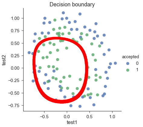
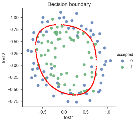
Draw decision boundary
- We find all the x satisfying x*theta=0Xtimestheta=0x*theta=0.
- instead of solving polynomial equation, just create a coridate x,y grid that is dense enough, and find all those X×θX\times \thetaX×θ that is close enough to 0, then plot them
def draw_boundary(power, l):
#     """
#     power: polynomial power for mapped feature
#     l: lambda constant
#     """
    density = 1000
    threshhold = 2 * 10**-3

    final_theta = feature_mapped_logistic_regression(power, l)
    x, y = find_decision_boundary(density, power, final_theta, threshhold)

    df = pd.read_csv('ex2data2.txt', names=['test1', 'test2', 'accepted'])
    sns.lmplot('test1', 'test2', hue='accepted', data=df, size=6, fit_reg=False, scatter_kws={"s": 100})

    plt.scatter(x, y, c='R', s=10)
    plt.title('Decision boundary')
    plt.show()
def feature_mapped_logistic_regression(power, l):
#     """for drawing purpose only.. not a well generealize logistic regression
#     power: int
#         raise x1, x2 to polynomial power
#     l: int
#         lambda constant for regularization term
#     """
    df = pd.read_csv('ex2data2.txt', names=['test1', 'test2', 'accepted'])
    x1 = np.array(df.test1)
    x2 = np.array(df.test2)
    y = get_y(df)

    X = feature_mapping(x1, x2, power, as_ndarray=True)
    theta = np.zeros(X.shape[1])

    res = opt.minimize(fun=regularized_cost,
                       x0=theta,
                       args=(X, y, l),
                       method='TNC',
                       jac=regularized_gradient)
    final_theta = res.x

    return final_theta
def find_decision_boundary(density, power, theta, threshhold):
    t1 = np.linspace(-1, 1.5, density)  #1000 samples
    t2 = np.linspace(-1, 1.5, density)

    cordinates = [(x, y) for x in t1 for y in t2]
    x_cord, y_cord = zip(*cordinates)
    mapped_cord = feature_mapping(x_cord, y_cord, power)  # this is a dataframe

    inner_product = mapped_cord.as_matrix() @ theta

    decision = mapped_cord[np.abs(inner_product) < threshhold]

    return decision.f10, decision.f01
#Finding Decision Boundary Functions
Change the value of lambda lambda lambda lambda lambda lambda lambda lambda lambda lambda lambda lambda lambda lambda lambda lambda lambda lambda lambda lambda lambda lambda lamb
draw_boundary(power=6, l=1) #set lambda = 1
draw_boundary(power=6,l=0) # set lambda < 0.1
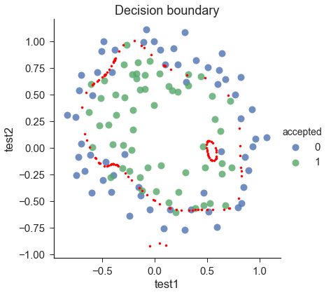
draw_boundary(power=6, l=100) # set lambda > 10