1 problems found

There are A simple linear regression model For example, paste the following content into the new test.py:

#Loading Library
import paddle.fluid as fluid
import numpy as np
#Generate data
np.random.seed(0)
outputs = np.random.randint(5, size=(10, 4))
res = []
for i in range(10):
        # Suppose the equation is y=4a+6b+7c+2d
        y = 4*outputs[i][0]+6*outputs[i][1]+7*outputs[i][2]+2*outputs[i][3]
        res.append([y])
# Defining data
train_data=np.array(outputs).astype('float32')
y_true = np.array(res).astype('float32')

#Defining network
x = fluid.layers.data(name="x",shape=[4],dtype='float32')
y = fluid.layers.data(name="y",shape=[1],dtype='float32')
y_predict = fluid.layers.fc(input=x,size=1,act=None)
#Define loss function
cost = fluid.layers.square_error_cost(input=y_predict,label=y)
avg_cost = fluid.layers.mean(cost)
#Define optimization methods
sgd_optimizer = fluid.optimizer.SGD(learning_rate=0.05)
sgd_optimizer.minimize(avg_cost)
#Parameter initialization
cpu = fluid.CPUPlace()
exe = fluid.Executor(cpu)
exe.run(fluid.default_startup_program())
##Start training, 500 iterations
for i in range(500):
        outs = exe.run(
                feed={'x':train_data,'y':y_true},
                fetch_list=[y_predict.name,avg_cost.name])
        if i%50==0:
                print ('iter={:.0f},cost={}'.format(i,outs[1][0]))
#Store training results
params_dirname = "result"
fluid.io.save_inference_model(params_dirname, ['x'], [y_predict], exe)

# Start forecasting
infer_exe = fluid.Executor(cpu)
inference_scope = fluid.Scope()
# Load the trained model
with fluid.scope_guard(inference_scope):
        [inference_program, feed_target_names,
         fetch_targets] = fluid.io.load_inference_model(params_dirname, infer_exe)

# Generate test data
test = np.array([[[9],[5],[2],[10]]]).astype('float32')
# Forecast
results = infer_exe.run(inference_program,
                                                feed={"x": test},
                                                fetch_list=fetch_targets)
# The output value of y=4*9+6*5+7*2+10*2 is given
print ("9a+5b+2c+10d={}".format(results[0][0]))

The operation results are as follows:

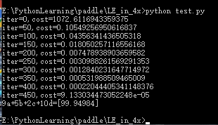
The learning effect is very good.

On the official website It is required to replace fluid.layers.data with fluid.data Therefore, the program is slightly changed:

1. Change fluid.layers.data to fluid.data

1.1 change the corresponding x shape to [- 1,4], and y shape to [- 1,1]

x = fluid.data(name="x",shape=[-1,4],dtype='float32')
y = fluid.data(name="y",shape=[-1,1],dtype='float32')

1.2 change the shape of test data to [1,4]

test = np.array([[9,5,2,10]]).astype('float32')

2. To increase the accuracy of the model, increase the training data from 10 groups to 20 groups

outputs = np.random.randint(5, size=(20, 4))
for i in range(20):

The modified code is as follows, save as test2.py

#Loading Library
import paddle.fluid as fluid
import numpy as np
#Generate data
np.random.seed(0)
outputs = np.random.randint(5, size=(20, 4))
res = []
for i in range(20):
        # Suppose the equation is y=4a+6b+7c+2d
        y = 4*outputs[i][0]+6*outputs[i][1]+7*outputs[i][2]+2*outputs[i][3]
        res.append([y])
# Defining data
train_data=np.array(outputs).astype('float32')
y_true = np.array(res).astype('float32')

#Defining network
x = fluid.data(name="x",shape=[-1,4],dtype='float32')
y = fluid.data(name="y",shape=[-1,1],dtype='float32')
y_predict = fluid.layers.fc(input=x,size=1,act=None)
#Define loss function
cost = fluid.layers.square_error_cost(input=y_predict,label=y)
avg_cost = fluid.layers.mean(cost)
#Define optimization methods
sgd_optimizer = fluid.optimizer.SGD(learning_rate=0.05)
sgd_optimizer.minimize(avg_cost)
#Parameter initialization
cpu = fluid.CPUPlace()
exe = fluid.Executor(cpu)
exe.run(fluid.default_startup_program())
##Start training, 500 iterations
for i in range(500):
        outs = exe.run(
                feed={'x':train_data,'y':y_true},
                fetch_list=[y_predict.name,avg_cost.name])
        if i%50==0:
                print ('iter={:.0f},cost={}'.format(i,outs[1][0]))
#Store training results
params_dirname = "result"
fluid.io.save_inference_model(params_dirname, ['x'], [y_predict], exe)

# Start forecasting
infer_exe = fluid.Executor(cpu)
inference_scope = fluid.Scope()
# Load the trained model
with fluid.scope_guard(inference_scope):
        [inference_program, feed_target_names,
         fetch_targets] = fluid.io.load_inference_model(params_dirname, infer_exe)

# Generate test data
test = np.array([[9,5,2,10]]).astype('float32')
# Forecast
results = infer_exe.run(inference_program,
                                                feed={"x": test},
                                                fetch_list=fetch_targets)
# The output value of y=4*9+6*5+7*2+10*2 is given
print ("9a+5b+2c+10d={}".format(results[0][0]))

The operation results are as follows:

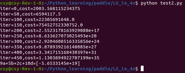
A strange thing happened: the increase of training data did not improve the performance of machine learning, but made it worse.

If you add data to 30 groups

outputs = np.random.randint(5, size=(30, 4))
for i in range(30):

The modified code is as follows, save as test3.py

#Loading Library
import paddle.fluid as fluid
import numpy as np
#Generate data
np.random.seed(0)
outputs = np.random.randint(5, size=(30, 4))
res = []
for i in range(30):
        # Suppose the equation is y=4a+6b+7c+2d
        y = 4*outputs[i][0]+6*outputs[i][1]+7*outputs[i][2]+2*outputs[i][3]
        res.append([y])
# Defining data
train_data=np.array(outputs).astype('float32')
y_true = np.array(res).astype('float32')

#Defining network
x = fluid.data(name="x",shape=[-1,4],dtype='float32')
y = fluid.data(name="y",shape=[-1,1],dtype='float32')
y_predict = fluid.layers.fc(input=x,size=1,act=None)
#Define loss function
cost = fluid.layers.square_error_cost(input=y_predict,label=y)
avg_cost = fluid.layers.mean(cost)
#Define optimization methods
sgd_optimizer = fluid.optimizer.SGD(learning_rate=0.05)
sgd_optimizer.minimize(avg_cost)
#Parameter initialization
cpu = fluid.CPUPlace()
exe = fluid.Executor(cpu)
exe.run(fluid.default_startup_program())
##Start training, 500 iterations
for i in range(500):
        outs = exe.run(
                feed={'x':train_data,'y':y_true},
                fetch_list=[y_predict.name,avg_cost.name])
        if i%50==0:
                print ('iter={:.0f},cost={}'.format(i,outs[1][0]))
#Store training results
params_dirname = "result"
fluid.io.save_inference_model(params_dirname, ['x'], [y_predict], exe)

# Start forecasting
infer_exe = fluid.Executor(cpu)
inference_scope = fluid.Scope()
# Load the trained model
with fluid.scope_guard(inference_scope):
        [inference_program, feed_target_names,
         fetch_targets] = fluid.io.load_inference_model(params_dirname, infer_exe)

# Generate test data
test = np.array([[9,5,2,10]]).astype('float32')
# Forecast
results = infer_exe.run(inference_program,
                                                feed={"x": test},
                                                fetch_list=fetch_targets)
# The output value of y=4*9+6*5+7*2+10*2 is given
print ("9a+5b+2c+10d={}".format(results[0][0]))

The operation results are as follows:

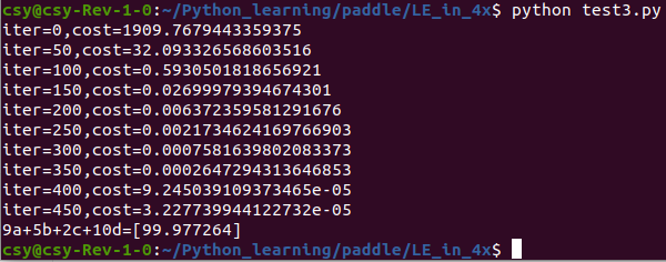
WOW! Academic performance has improved again. Better than 10 sets of data training.

2 find problems

In order to find out the problem, some modifications and simplifications have been made to the program:

1. Instead, input numbers with keyboard to determine the number of groups and generate training data
2. Change to use the keyboard to input numbers to determine the generated training data range
3. Change to use keyboard to input numbers to determine random seeds
5. Randomly generate training data of floating-point numbers
6. Print out training data
7. Do not save model
8. Delete the test part

The modified code is as follows, save as test7.py

#Loading Library
import paddle.fluid as fluid
import numpy as np

#Generate data
group = input('Enter a positive integer to determine the amount of data generated:')
group = int(group)
data_range = input('Please enter a positive integer to determine the value range of training data generated:')
float_range = float(data_range)
random_seed = input('Please enter a positive integer as the seed of the random number:')

np.random.seed(int(random_seed))
outputs =np.random.uniform(1,float_range,size=(group,4)) #float64

res = []  #Generate an empty list
for i in range(group):
    #If the equation is y=4a+6b+7c+2d, the answer will be generated
    y = 4*outputs[i][0]+6*outputs[i][1]+7*outputs[i][2]+2*outputs[i][3]
    print("{}: {}=({},{},{},{})".format(i,y,outputs[i][0],outputs[i][1],outputs[i][2],outputs[i][3]))
    res.append([y])  # When the variable is array [] [], the corresponding y value is saved in res

# Defining data
train_data = np.array(outputs).astype('float32')   # The training data uses 10 groups of randomly generated data to change the integer random number to floating-point type
y_true = np.array(res).astype('float32')           # Corresponding standard answer
print(train_data.shape,y_true.shape)

# Defining network
x = fluid.data(name="x",shape=[None,4],dtype='float32')
y = fluid.data(name="y",shape=[None,1],dtype='float32')
y_predict = fluid.layers.fc(input=x,size=1,act=None)

# Define loss function
cost = fluid.layers.square_error_cost(input=y_predict,label=y)
avg_cost = fluid.layers.mean(cost)

# Definition optimization
sgd_optimizer = fluid.optimizer.SGD(learning_rate=0.05)
sgd_optimizer.minimize(avg_cost)

#Parameter initialization
cpu = fluid.CPUPlace()
exe = fluid.Executor(cpu)
exe.run(fluid.default_startup_program())

## Start training, 500 iterations
for i in range(500):
    outs = exe.run(
        feed={'x':train_data,'y':y_true},
        fetch_list=[y_predict.name,avg_cost.name])
    if i%50==0:
        print('iter={:.0f},cost={}'.format(i,outs[1][0]))

First run:

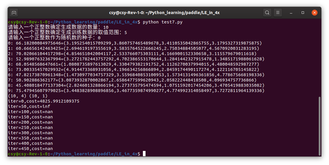
Second operation:

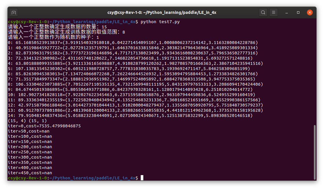
Change learning rate to 001

sgd_optimizer = fluid.optimizer.SGD(learning_rate=0.01)

Operation result:

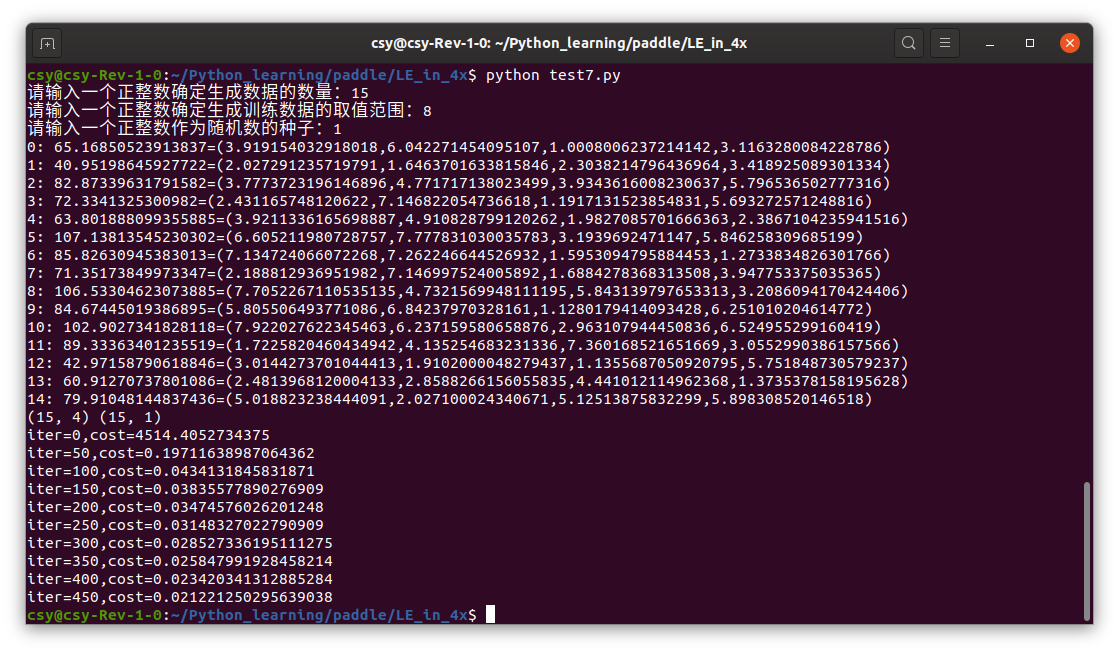
Then change the learning rate of test2.py to 0.01, and the running result is as follows:

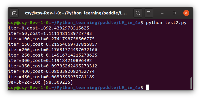
After the decrease of learning rate, every training has improved, but not much. But not backward.

3 my conclusion

The shape and type of training data must be consistent with the shape and type of fluid.data. The shape and type of training data must also be consistent with the shape and type of fluid.data.

The high learning rate is equivalent to the jump of students. If it goes well, I will study faster than other students and graduate early. But it may not be as good as the step-by-step students, that is to say, there is a risk of pulling up the weak and encouraging the weak. The learning rate is low, and we can make progress day by day. It is necessary to adjust the stability and speed.

The range of training data should preferably cover the range of test data. If the test questions are told by the teacher in class, the test results will be better.

The larger the number of training data, the more beautiful the value of loss function. If not, consider whether the learning rate needs to be lowered.