Catalog
1. Activation function
The idea of activation function comes from the analysis of the working mechanism of neurons in human brain. Neurons are activated above a certain threshold (also known as activation potential). In most cases, the activation function is also intended to limit the output to a small range.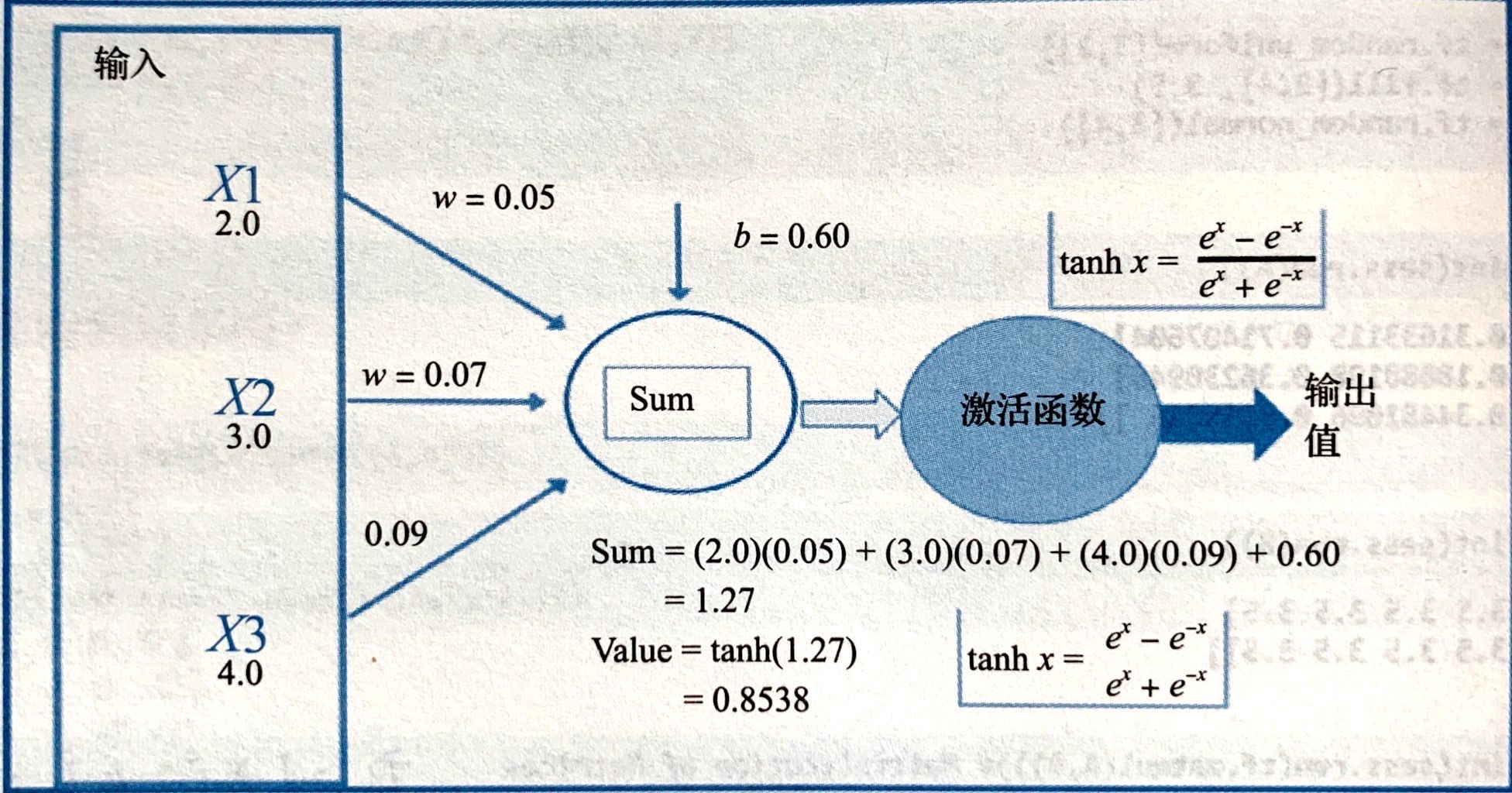
1.1 hyperbolic tangent function and Sigmoid function
The following figure shows the tanh and Sigmoid activation functions: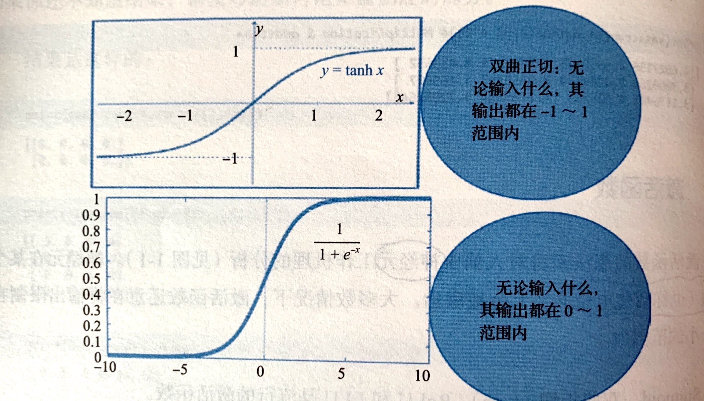
The demo code is as follows: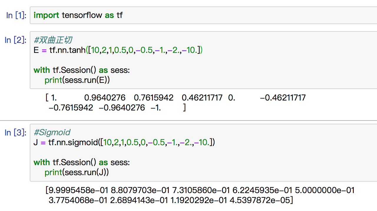
2. Loss function (cost function)
The loss function (cost function) is used to minimize to get the optimal value of each parameter of the model. For example, in order to use the predictor (X) to predict the value of the target (y), it is necessary to obtain the weight value (slope) and the offset amount (y intercept). The method to get the optimal value of slope and Y intercept is to minimize the sum of cost function / loss function / square. For any model, there are many parameters, and the model structure of prediction or classification is also represented by the value of parameters.
You need to calculate the model, and to do that, you need to define a cost function (loss function). The purpose of minimizing loss function is to find the optimal value of each parameter. L1 or L2 are useful loss functions for regression / numerical prediction problems. For classification problems, cross entropy is a very useful loss function. Softmax or Sigmoid cross entropy are very popular loss functions
2.1 L1 norm loss function
The L1 norm loss function, also known as the least absolute deviation (LAD), the least absolute error (LAE). In general, it is to minimize the sum (S) of the absolute difference between the target value (Yi) and the estimated value (f(xi)):
2.2 L2 norm loss function
L2 norm loss function, also known as least square error (LSE). In general, it is to minimize the sum of squares (S) of the difference between the target value (Yi) and the estimated value (f(xi)):
2.3 quadratic cost function

C is the cost function, x is the sample, y is the actual value, a is the output value, and n is the total number of samples.
For the sake of simplicity, take the example of only one sample,
a=σ(z), z=∑Wj*Xj+b
σ () is the activation function
In this case, the quadratic cost function is: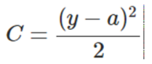
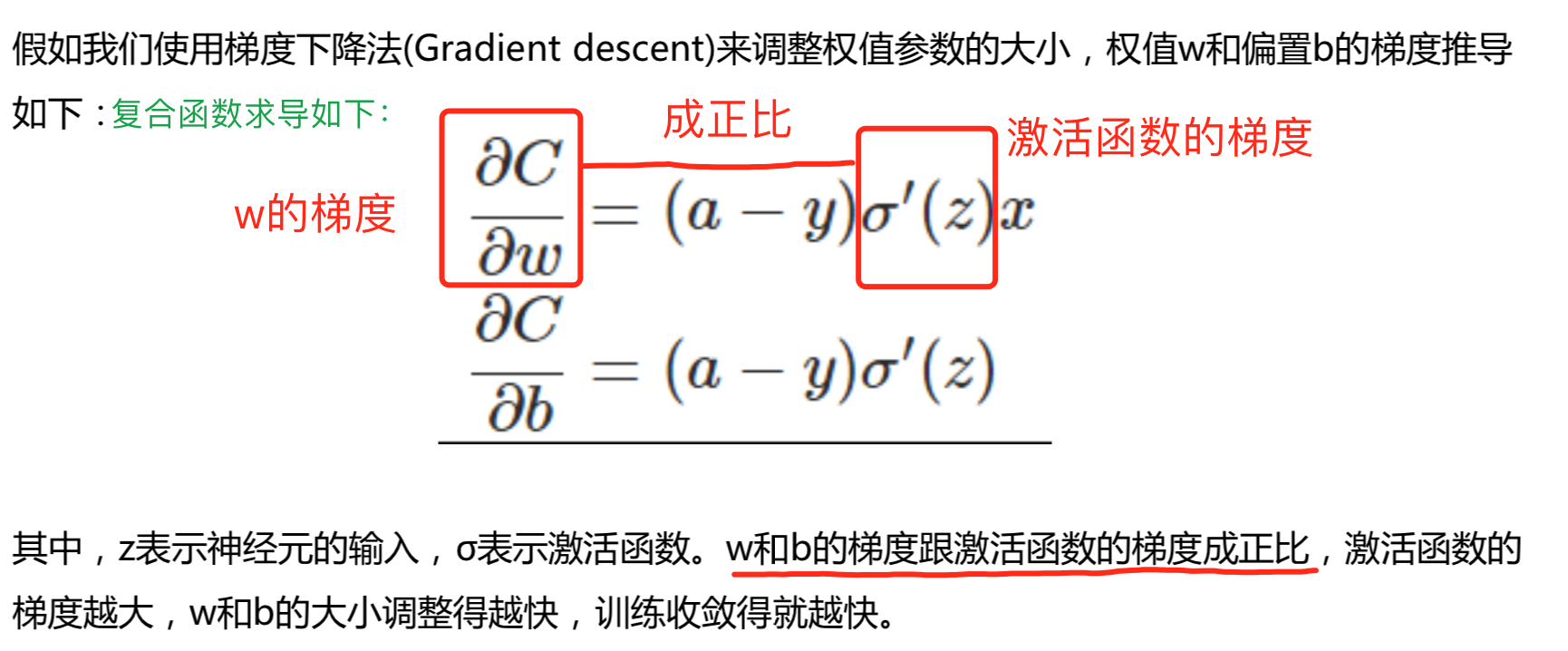
It can be seen from the above that the gradient change of the quadratic cost function W and b is related to the activation function.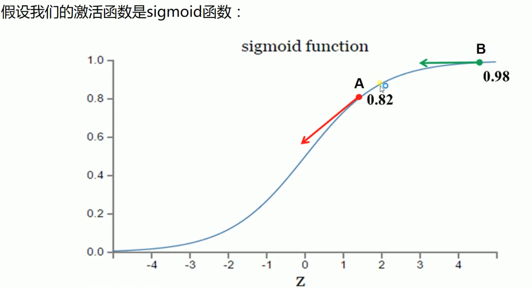
- Let's suppose that our goal of convergence is 1. Point A is 0.82, which is far away from the target, while point A has A larger gradient and A larger weight adjustment. Point B is 0.98, which is close to the target, while point B has A smaller gradient and A smaller weight adjustment. Therefore, it can quickly adjust from point A to point B, and then slowly converge to point 1. This scheme is reasonable.
- Let's suppose that our goal of convergence is 0. Point B is 0.98, which is far away from the target, while point B has A smaller gradient and smaller weight adjustment. Point A is 0.82, which is close to the target, while point A has A larger gradient and larger weight adjustment. Therefore, if it starts from point B, it will take A long time to reach point A at point B, then this scheme is unreasonable.
If the error is relatively large, it means that we are far away from our goal. At this time, the weight adjustment should be relatively large, which we think is more reasonable.
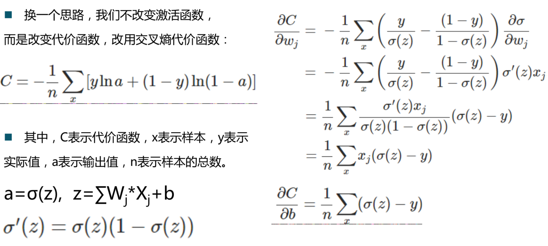
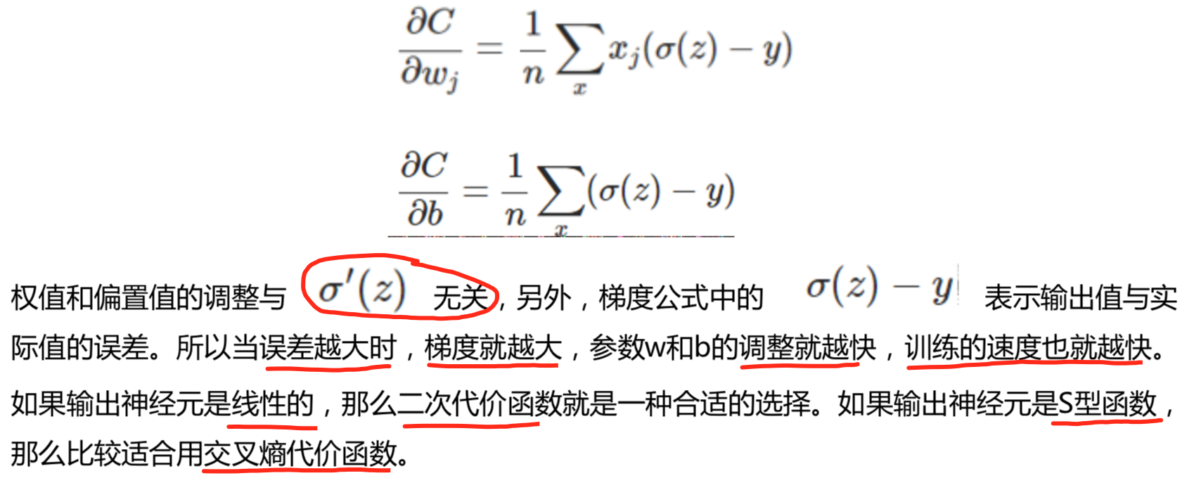
2.4 cross entropy cost function
2.5 log likelihood cost
Logarithmic relief function is often used as the cost function of softmax regression. If the output layer neuron is sigmoid function, cross entropy cost function can be used. In depth learning, softmax is regarded as the last layer. At this time, the common cost function is the logarithmic release cost function.
The combination of log likelihood cost function and softmax, and the combination of cross entropy and sigmoid function are very similar. The logarithmic release cost function can be reduced to the form of cross entropy cost function in binary classification.
In Tensorflow, use:
TF. NN. Sigmoid? Cross? Entropy? With? Logits() to represent the cross entropy used with sigmoid. TF. NN. Softmax? Cross? Entropy? With? Logits() to represent the cross entropy used with softmax.
3. Demo code
Modify 3-2 to simply implement handwritten digit recognition code, and use softmax cross entropy cost function:
import tensorflow as tf
from tensorflow.examples.tutorials.mnist import input_data
#Load data set
mnist = input_data.read_data_sets("MNIST_data",one_hot=True)

#Size of each batch
batch_size = 50
#How many batches are there
n_batch = mnist.train.num_examples // batch_size

#Define two placeholder s
x = tf.placeholder(tf.float32,[None,784])
y = tf.placeholder(tf.float32,[None,10])

#Create a simple neural network
W = tf.Variable(tf.zeros([784,10]))
b = tf.Variable(tf.zeros([10]))
prediction = tf.nn.softmax(tf.matmul(x,W) + b)

#Quadratic cost function
# loss = tf.reduce_mean(tf.square(y-prediction))
#Using softmax cross entropy cost function
loss = tf.reduce_mean(tf.nn.softmax_cross_entropy_with_logits(labels=y,logits=prediction))
#Training with gradient descent method
train_step = tf.train.GradientDescentOptimizer(0.2).minimize(loss)

#initialize variable
init = tf.global_variables_initializer()

#Results are stored in a Boolean list
#argmax returns the position of the maximum value in one-dimensional tensor
correct_prediction = tf.equal(tf.argmax(y,1),tf.argmax(prediction,1))
#Accuracy rate
accuracy = tf.reduce_mean(tf.cast(correct_prediction,tf.float32))

with tf.Session() as sess:
    sess.run(init)
    for epoch in range(21):
        for batch in range(n_batch):
            batch_xs,batch_ys = mnist.train.next_batch(batch_size)
            sess.run(train_step,feed_dict = {x:batch_xs,y:batch_ys})

        acc = sess.run(accuracy,feed_dict = {x:mnist.test.images,y:mnist.test.labels})
        print("Iter"+str(epoch)+",Testing Accuracy"+str(acc))
Comparison of operation results
#The result of quadratic cost function
Iter0,Testing Accuracy0.8703
Iter1,Testing Accuracy0.8876
Iter2,Testing Accuracy0.8964
Iter3,Testing Accuracy0.9018
Iter4,Testing Accuracy0.9047
Iter5,Testing Accuracy0.9069
Iter6,Testing Accuracy0.9094
Iter7,Testing Accuracy0.9108
Iter8,Testing Accuracy0.9121
Iter9,Testing Accuracy0.9135
Iter10,Testing Accuracy0.9145
Iter11,Testing Accuracy0.9155
Iter12,Testing Accuracy0.9166
Iter13,Testing Accuracy0.9176
Iter14,Testing Accuracy0.9176
Iter15,Testing Accuracy0.9183
Iter16,Testing Accuracy0.9186
Iter17,Testing Accuracy0.9192
Iter18,Testing Accuracy0.9195
Iter19,Testing Accuracy0.919
Iter20,Testing Accuracy0.9205
#Result of cross entropy cost function
Iter0,Testing Accuracy0.8944
Iter1,Testing Accuracy0.9054
Iter2,Testing Accuracy0.9099
Iter3,Testing Accuracy0.9134
Iter4,Testing Accuracy0.9148
Iter5,Testing Accuracy0.9167
Iter6,Testing Accuracy0.9202
Iter7,Testing Accuracy0.9207
Iter8,Testing Accuracy0.9211
Iter9,Testing Accuracy0.9214
Iter10,Testing Accuracy0.9214
Iter11,Testing Accuracy0.9222
Iter12,Testing Accuracy0.9228
Iter13,Testing Accuracy0.9237
Iter14,Testing Accuracy0.924
Iter15,Testing Accuracy0.9245
Iter16,Testing Accuracy0.9238
Iter17,Testing Accuracy0.9245
Iter18,Testing Accuracy0.9244
Iter19,Testing Accuracy0.9251
Iter20,Testing Accuracy0.9251
It can be seen from the results that when the accuracy reaches 0.909, it needs 6 iterations to use the quadratic cost function, and only 2 iterations to use the softmax cross entropy function. It is obvious that the speed of using the cross entropy cost function will be much faster.
conclusion
So when we use S-type activation function or softmax, we should use cross entropy cost function, which is more efficient.

