Boston House Price Prediction:Optimization Based on Normal Equation and Gradient Decline
Data Code Download Address
Project Link + Source Code: https://github.com/w1449550206/Boston-house-price-forecast.git
Article Directory
- Boston House Price Prediction:Optimization Based on Normal Equation and Gradient Decline
- Data Code Download Address
- Data introduction
- Detailed steps
- [Linear Regression Optimized by Normal Equation]
- 1. Get data load_boston
- 2. Basic Data Processing Divides Datasets and Test Sets
- 3. Standardization of Feature Engineering
- 4. Machine learning linear regression (normal equation optimization, gradient descent optimization)
- 4.1 Create model instantiation estimator
- 4.2 Training Model fit Normal Equation Calculates Optimal Trainable Parameters
- 5. Model evaluation MSE (mean square error, smaller is better) Both predicted and true values are required
- [Linear regression with gradient descent optimization]
- 1. Get data load_boston
- 2. Basic Data Processing Divides Datasets and Test Sets
- 3. Standardization of Feature Engineering
- 4. Machine learning linear regression (normal equation optimization, gradient descent optimization)
- 4.1 Create model instantiation estimator
- 4.2 Training Model fit Normal Equation Calculates Optimal Trainable Parameters
- 5. Model evaluation MSE (mean square error, smaller is better) Both predicted and true values are required
Data introduction
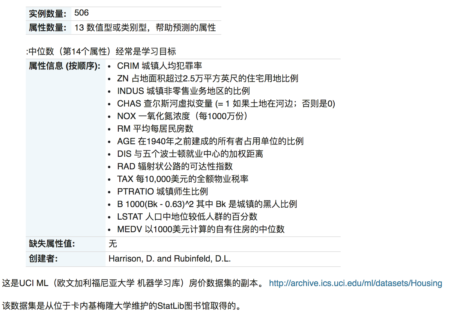
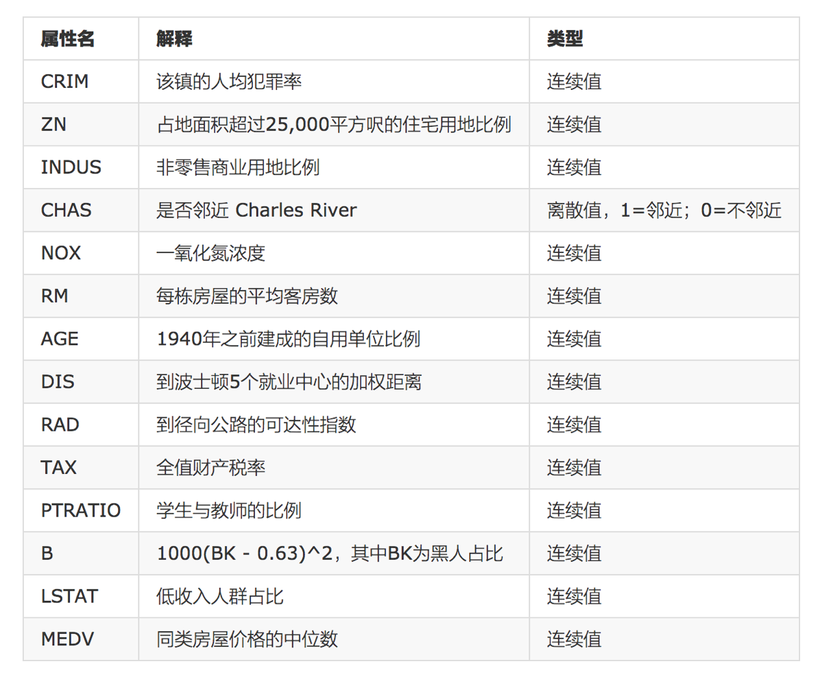
Given these characteristics, they are the result attributes that experts derive to influence house prices.We don't need to explore the usefulness of features by ourselves at this stage, just use them.Quantifying many features later requires us to look for them ourselves
1 Analysis
Whether inconsistent data sizes in regression will result in greater impact on results.So standardization is needed.
- Data segmentation and standardization
- Regression Prediction
- Evaluation of Algorithmic Effect of Linear Regression
2 Regression performance evaluation
Mean Squared Error MSE evaluation mechanism:
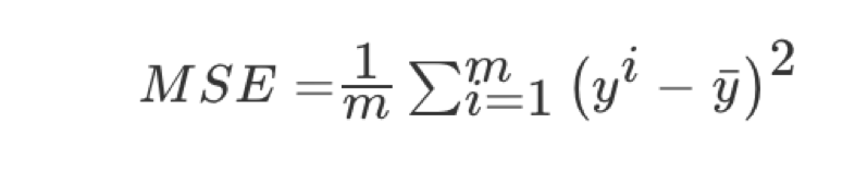
Note: yi is the predicted value and y is the true value
- sklearn.metrics.mean_squared_error(y_true, y_pred)
- Mean Square Error Regression Loss
- y_true:true value
- y_pred:Predicted value
- return:floating point result
Detailed steps
#Packages to use
from sklearn.datasets import load_boston
from sklearn.model_selection import train_test_split
from sklearn.preprocessing import StandardScaler
from sklearn.linear_model import LinearRegression
from sklearn.metrics import mean_squared_error
from sklearn.linear_model import SGDRegressor
[Linear Regression Optimized by Normal Equation]
1. Get data load_boston
data = load_boston()
2. Basic Data Processing Divides Datasets and Test Sets
x_train,x_test,y_train,y_test = train_test_split(data.data, data.target,test_size = 0.2, random_state = 10)#random_state = 10 guarantees the same division of datasets
3. Standardization of Feature Engineering
#Using interface standardscaler
transfer  = StandardScaler()
x_train = transfer.fit_transform(x_train)
x_test = transfer.fit_transform(x_test)
4. Machine learning linear regression (normal equation optimization, gradient descent optimization)
4.1 Create model instantiation estimator
estimator = LinearRegression()
4.2 Training Model fit Normal Equation Calculates Optimal Trainable Parameters
estimator.fit(x_train,y_train)

5. Model evaluation MSE (mean square error, smaller is better) Both predicted and true values are required
5.1 Getting Predicted Values
y_predict = estimator.predict(x_test)
5.2 Computing MSE
mean_squared_error(y_pred=y_predict,y_true=y_test)#The mean square error is obtained, the smaller the better

[Linear regression with gradient descent optimization]
1. Get data load_boston
data = load_boston()
2. Basic Data Processing Divides Datasets and Test Sets
x_train,x_test,y_train,y_test = train_test_split(data.data, data.target,test_size = 0.2, random_state = 10)#random_state = 10 guarantees the same division of datasets
3. Standardization of Feature Engineering
#Using interface standardscaler
transfer  = StandardScaler()
x_train = transfer.fit_transform(x_train)
x_test = transfer.fit_transform(x_test)
4. Machine learning linear regression (normal equation optimization, gradient descent optimization)
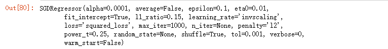
4.1 Create model instantiation estimator
estimator = SGDRegressor(max_iter=1000,tol=0.001)#tol=0.001 refers to whether the loss function is getting smaller and smaller for each iteration and stops iteration if the value of the loss function is less than 0.001
4.2 Training Model fit Normal Equation Calculates Optimal Trainable Parameters
estimator.fit(x_train,y_train)
5. Model evaluation MSE (mean square error, smaller is better) Both predicted and true values are required
5.1 Getting Predicted Values
y_predict = estimator.predict(x_test)
5.2 Computing MSE
mean_squared_error(y_pred=y_predict,y_true=y_test)#The mean square error is obtained, the smaller the better

We can also try to modify the learning rate
estimator = SGDRegressor(max_iter=1000,learning_rate="constant",eta0=0.1)
At this time, we can find a better value of learning rate by adjusting parameters.

