View data

import numpy as np
import pandas as pd
import matplotlib.pyplot as plt

data=pd.read_csv("code/ex2-logistic regression/ex2data1.txt",names=['Exam 1', 'Exam 2', 'Admitted'])
data.head()

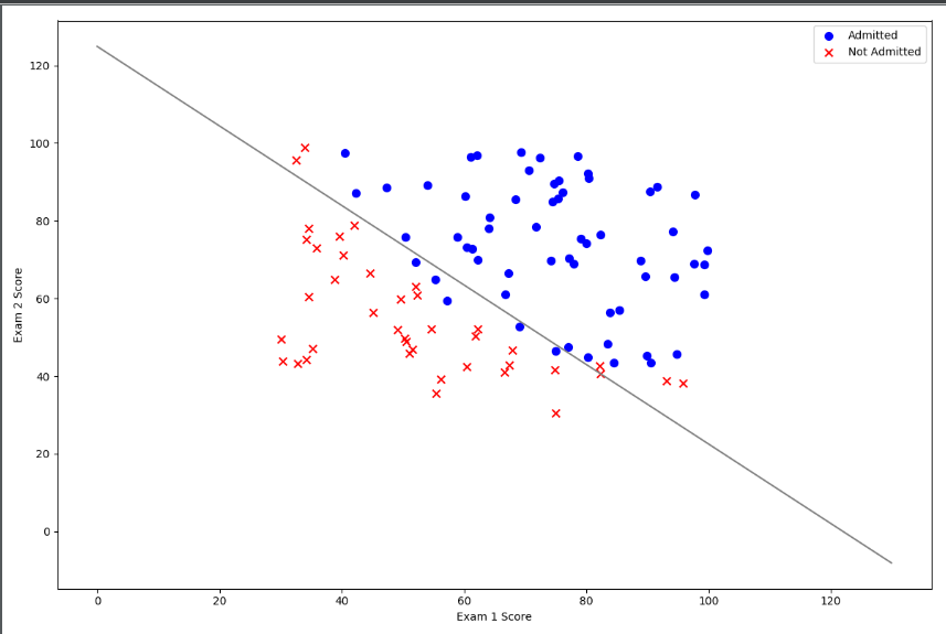
positive=data[data["Admitted"].isin(["1"])]
negative=data[data["Admitted"].isin(["0"])]
fig,ax=plt.subplots(figsize=[12,8])
ax.scatter(positive['Exam 1'], positive['Exam 2'], s=50, c='b', marker='o', label='positive')
ax.scatter(negative['Exam 1'], negative['Exam 2'], s=50, c='r', marker='x', label='negative')
ax.legend()
ax.set_xlabel('Exam 1 Score')
ax.set_ylabel('Exam 2 Score')
plt.show()

About pandas.isin() A kind of :
isin() accepts a list and determines whether the elements in the column are in the list.
Give an example:

>>> df
          A         B         C         D  E
0 -0.018330  2.093506 -0.086293 -2.150479  a
1  0.104931 -0.271810 -0.054599  0.361612  a
2  0.590216  0.218049  0.157213  0.643540  c
3 -0.254449 -0.593278 -0.150455 -0.244485  b
>>> df.E.isin(['a','c'])
0     True
1     True
2     True
3    False
Name: E, dtype: bool
--------
Copyright notice: This is the original article of CSDN blogger "lzw2016", following CC 4.0 BY-SA copyright agreement. Please attach the original source link and this notice for reprint.
Original link: https://blog.csdn.net/lzw2016/article/details/80472649

After data visualization:

sigmoid function

def sigmoid(z):
    return 1/(1+np.exp(-z))

Cost function

For linear regression models, the error we define is the sum of the squares of all model errors:
But for the logistic regression model, theBy substituting the above cost function, we will get a nonconvex function, which leads to many local minima in our cost function, which will affect the gradient descent algorithm to find the global minima.
So we redefine the cost function:

data.insert(0,"ones",1)#Add a column x0=1 so that the number of X is the same as theta
cols=data.shape[1]
X=data.iloc[:,0:cols-1]
Y=data.iloc[:,cols-1:cols]
X=np.array(X.values)
Y=np.array(Y.values)
theta=np.zeros(3)

def cost(theta,X,Y):
    theta=np.matrix(theta)
    z=np.dot(X,theta.T)
    m=len(X)
    cost=1/m*np.sum(np.multiply(-Y,np.log(sigmoid(z)))-np.multiply((1-Y),np.log(1-sigmoid(z))))
    return cost

cost(theta,X,Y)

theta=np.matrix(theta) changes theta from (3,) to (3, 1)
The former is one-dimensional, the latter is two-dimensional.
For example:
The result of NP. Sum (two-dimensional matrix, axis=1) is one-dimensional
NP. Sum (two-dimensional matrix, axis=1,keepdims=True) results in two-dimensional
On the difference between Python list, Numpy array and matrix

gradient descent

def gradient(theta,X,Y):
    theta = np.matrix(theta)
    X = np.matrix(X)
    Y = np.matrix(Y)
    parameters=int(theta.ravel().shape[1])
    grads=np.zeros(parameters)
    z=np.dot(X,theta.T)
    error=sigmoid(z)-Y
    for i in range(parameters):
        term=np.multiply(error,X[:,i])
        grads[i]=np.sum(term)/len(X)
    return grads
gradient(theta,X,Y)                     

Note that we are not actually performing gradient descent in this function, we are only calculating a gradient step. In the exercise, an Octave function called "fminunc" is used to optimize the function to calculate the cost and gradient parameters. Because we use Python, we can do the same with SciPy's "optimize" namespace.

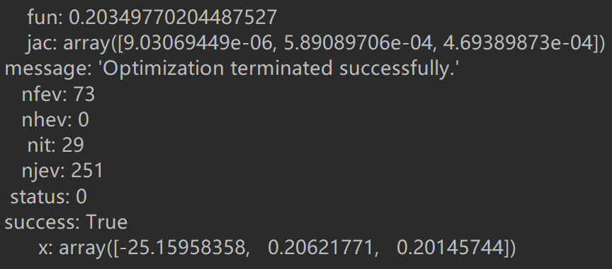
import scipy.optimize as opt
res = opt.minimize(fun=cost, x0=theta, args=(X, Y), method='Newton-CG', jac=gradient)
print(res)

About scipy.optimize:

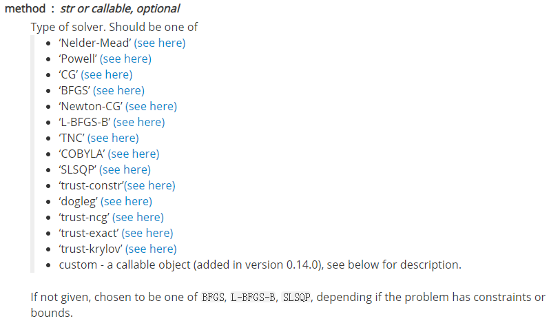
scipy.optimize.minimize(fun, x0, args=(), method=None, jac=None, hess=None, hessp=None, bounds=None, constraints=(), tol=None, callback=None, options=None)[source]¶

• fun: minimized objective function
• x0: initialized parameters
• args: parameters passed to the target function
• Optimization method:
• bounds: limits on variables for l-bfgs-b, TNC, slsqp and
  trust-constr methods.)
• Constraints: Constraints definition (only for COBYLA, SLSQP and
  trust-constr)
  ......
  scipy.optimize.minimize

Forecast

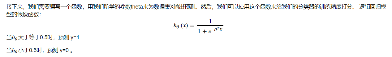
def predict(theta, X):
    z=np.dot(X,theta.T)
    probs = sigmoid(z)
    return [1 if x >= 0.5 else 0 for x in probs]

theta_min = np.matrix(res.x)
predictions = predict(theta_min, X)
correct = [1 if ((a == 1 and b == 1) or (a == 0 and b == 0)) else 0 for (a, b) in zip(predictions, Y)]
accuracy = (sum(map(int, correct)) % len(correct))
print ('accuracy = {0}%'.format(accuracy))

accuracy = 89%

Drawing decision boundaries

coef = -(res.x / res.x[2])  # find the equation
print(coef)

x = np.arange(130, step=0.1)
y = coef[0] + coef[1]*x
data.describe()  # find the range of x and y

coef[0] is intercept, about 125

fig, ax = plt.subplots(figsize=(12,8))
ax.scatter(positive['Exam 1'], positive['Exam 2'], s=50, c='b', marker='o', label='Admitted')
ax.scatter(negative['Exam 1'], negative['Exam 2'], s=50, c='r', marker='x', label='Not Admitted')
ax.plot(x,y,'grey')
ax.legend()
ax.set_xlabel('Exam 1 Score')
ax.set_ylabel('Exam 2 Score')
plt.show()