preface

Original translation from: Deep Learning with PyTorch: A 60 Minute Blitz

Translation: Lin Yun

catalogue

60 minute introduction to PyTorch (I) - Tensors

60 minute introduction to PyTorch (II) -- Autograd automatic derivation

60 minute introduction to pytoch (III) -- neural network

60 minute introduction to PyTorch (IV) -- training a classifier

%matplotlib inline

Train a classifier

You have learned how to define a neural network, calculate the loss value and update the weight of the network.

You may be thinking now: where does the data come from?

jupyter nbconvert --to md notebook.ipynb

About data

Usually, when you process image, text, audio and video data, you can use the standard Python package to load the data into a numpy array Then convert this array to torch* Tensor.

• For images, there are very practical packages such as pilot and OpenCV
• For audio, there are packages such as scipy and librosa
• For text, you can load it with raw Python and python, or use NLTK and SpaCy
  For vision, we created a torchvision package, which contains data loading of common data sets, such as Imagenet,CIFAR10,MNIST, etc., and image converter, that is, torchvision Datasets and torch utils. data. DataLoader.

This provides great convenience and avoids code duplication.

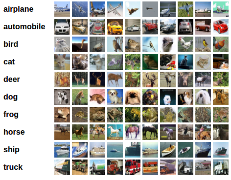
In this tutorial, we use CIFAR10 dataset, which has the following 10 categories: 'airplane', 'automobile', 'bird', 'cat', 'der', 'dog', 'frog', 'horse', 'ship', 'truck'. The image size in this dataset is 3 * 32 * 32, that is, 3 channels, 32 * 32 pixels.

Training an image classifier

We will proceed in the following order:

• Use torchvision to load and normalize CIFAR10 training set and test set
• A convolutional neural network is defined
• Define loss function
• Training network on training set
• Test network on test set

1. Loading and normalizing CIFAR10

Loading CIFAR10 using torchvision is very easy.

import torch

import torchvision

import torchvision.transforms as transforms

The output of torchvision is the PILImage of [0,1], which we convert into a tensor with a normalized range of [- 1,1].

transform = transforms.Compose(

    [transforms.ToTensor(),

     transforms.Normalize((0.5, 0.5, 0.5), (0.5, 0.5, 0.5))])



trainset = torchvision.datasets.CIFAR10(root='./data', train=True,

                                        download=True, transform=transform)

trainloader = torch.utils.data.DataLoader(trainset, batch_size=4,

                                          shuffle=True, num_workers=2)



testset = torchvision.datasets.CIFAR10(root='./data', train=False,

                                       download=True, transform=transform)

testloader = torch.utils.data.DataLoader(testset, batch_size=4,

                                         shuffle=False, num_workers=2)



classes = ('plane', 'car', 'bird', 'cat',

           'deer', 'dog', 'frog', 'horse', 'ship', 'truck')

#This process is a little slow. About 340mb of image data will be downloaded.

Files already downloaded and verified
Files already downloaded and verified

We show some interesting training images.

import matplotlib.pyplot as plt

import numpy as np

import cv2



# functions to show an image





def imshow(img):

    img = img / 2 + 0.5     # unnormalize

    npimg = img.numpy()

    

    suofanghou=cv2.resize(np.transpose(npimg, (1, 2, 0)),(640,440),interpolation=cv2.INTER_CUBIC)

    cv2.imshow("img",suofanghou)

    cv2.waitKey(0)

    # plt.imshow(np.transpose(npimg, (1, 2, 0)))

    # plt.show()





# get some random training images

dataiter = iter(trainloader)

images, labels = dataiter.next()

# print(images)

# print(labels)



# show images

# images = torchvision.utils.make_grid(images)

# array1=images.numpy()#Convert tensor data to numpy data

# maxValue=array1.max()

# array1=array1*255/maxValue#normalize to expand the image data to [0255]

# mat=np.uint8(array1)#float32-->uint8

# print('mat_shape:',mat.shape)#mat_shape: (3, 982, 814)

# mat=mat.transpose(1,2,0)#mat_shape: (982, 814，3)

# cv2.imshow("img",mat)

# cv2.waitKey(0)

imshow(torchvision.utils.make_grid(images))

# print labels

print(' '.join('%5s' % classes[labels[j]] for j in range(4)))

 bird   car  bird   dog

2. Define a convolutional neural network

Copy the neural network code from the previous neural network section and modify it to accept the 3-channel image instead of the previous single channel image.

import torch.nn as nn

import torch.nn.functional as F



# Function of convolution layer: feature extraction of input pictures.

# The input image is convoluted with the kernel to obtain the output.

# Note: the number of cores should be consistent with the number of input channel s. A kernel is convoluted with only one channel.

# The role of the pool layer is to reduce the size of the input picture.

# In convolutional neural networks, each convolution layer is always followed by a pool layer.

# The function of adding pooling layer is to speed up the operation and make some detected features more robust.

# The full connection layer appears at the end of the convolutional neural network.

# Before the fully connected layer, the feature map generated by many previous layers is compressed into a vector. This vector is fed into the full connection layer.

# The output of the full connection layer is a one-dimensional eigenvector.

class Net(nn.Module):

    def __init__(self):

        super(Net, self).__init__()

        # [ channels, output, height_2, width_2 ]

        # Channels, the number of channels, is consistent with the above, that is, the depth of the current layer

        # Depth of output

        # height_2. filter height

        # width_2. Width of filter

        # Convolution layer 1: two-dimensional convolution layer, 3 input channels and 6 output channels, and the size of convolution kernel is 5x5

        self.conv1 = nn.Conv2d(3, 6, 3)

        # pool of square window of size=2, stride=2

        # Maximum pool layer

        self.pool = nn.MaxPool2d(2, 2)

        # Convolution layer 2: two-dimensional convolution layer, 6 input channels and 16 output channels, with convolution kernel size of 5x5

        self.conv2 = nn.Conv2d(6, 16, 3)

        # self.pool2 = nn.MaxPool2d(2, 2)

        # self.conv3 = nn.Conv2d(16, 36, 3)

        # For the full connection layer, it should be noted that the input and output of the full connection layer are two-dimensional tensors, and the general shape is [batch_size, size]

        # in_features refers to the size of the input two-dimensional tensor, that is, the size in the input [batch_size, size].

        # out_features refers to the size of the output two-dimensional tensor, that is, the shape of the output two-dimensional tensor is [batch_size, output_size]

        # in_features are determined by the shape of the input tensor, out_features determine the shape of the output tensor 

        # nn.Linear(in_features = 16 * 5 * 5, out_features = 120)

        # /*

        # The number of input features for a linear layer is defined by the active dimension from the previous layer.

        # The active shape of the upper layer is [batch_size, channels= 16, height= 5, width= 5].

        # To pass this activation to NN Linear, you need to flatten this tensor to [batch_size, 16 * 5 * 5].

        # 16 By out_ The number of channels (i.e. the number of filter cores in the previous conv layer) is defined,

        # 5x5 is the size of the space defined by the conv and the pooling operation performed on the input data.

        # */

        # An affine operation: y = Wx + b 

        # # Full connection layer 1: linear layer, input dimension 16 * 5 * 5, output dimension 120

        self.fc1 = nn.Linear(16 * 6 * 6, 120)

        # Full connection layer 2: linear layer, input dimension 120, output dimension 84

        self.fc2 = nn.Linear(120, 84)

        # Full connection layer 3: linear layer, input dimension 84, output dimension 10

        self.fc3 = nn.Linear(84, 10)



    def forward(self, x):

        #  # Convolution first, then pooling

        x = self.pool(F.relu(self.conv1(x)))

        # Re convolution

        x = self.pool(F.relu(self.conv2(x)))

        # When changing the convolution and size and reporting an error, check the size of the feature map. The size is torch Size([4, 16, 6, 6])，

        # In fact, the size of your feature map is 16 * 6 * 6, and the input dimension is 16 * 6 * 6

        # Expected input batch_size (16) to match target batch_size (4).

        # print(x.shape)

        x = x.view(-1, 16 * 6 * 6)

        # Full connection 1

        x = F.relu(self.fc1(x))

        # Full connection 2

        x = F.relu(self.fc2(x))

        x = self.fc3(x)

        return x





net = Net()

print(net)

Net(
  (conv1): Conv2d(3, 6, kernel_size=(3, 3), stride=(1, 1))
  (pool): MaxPool2d(kernel_size=2, stride=2, padding=0, dilation=1, ceil_mode=False)
  (conv2): Conv2d(6, 16, kernel_size=(3, 3), stride=(1, 1))
  (fc1): Linear(in_features=576, out_features=120, bias=True)
  (fc2): Linear(in_features=120, out_features=84, bias=True)
  (fc3): Linear(in_features=84, out_features=10, bias=True)
)

3. Define loss function and optimizer

We use the cross entropy as the loss function and the random gradient descent of the driving quantity.

import torch.optim as optim



criterion = nn.CrossEntropyLoss()

#list(net.parameters()) will give a parameter list, recording the data of all training parameters (W and b)

optimizer = optim.SGD(net.parameters(), lr=0.001, momentum=0.9)

4. Training network

This is the first interesting moment. We just need to loop on the data iterator, input the data into the network and optimize it.

for epoch in range(2):  # loop over the dataset multiple times



    running_loss = 0.0

    for i, data in enumerate(trainloader, 0):

        # get the inputs; data is a list of [inputs, labels]

        inputs, labels = data



        # 4 initialization: clear the cache, calculate the gradient, and set the optimizer

        # zero the parameter gradients

        optimizer.zero_grad()



        # forward + backward + optimize

        outputs = net(inputs)

        loss = criterion(outputs, labels)

        loss.backward()

        optimizer.step()



        # print statistics

        running_loss += loss.item()

        if i % 2000 == 1999:    # print every 2000 mini-batches

            print('[%d, %5d] loss: %.3f' %

                  (epoch + 1, i + 1, running_loss / 2000))

            running_loss = 0.0



print('Finished Training')

[1,  2000] loss: 2.218
[1,  4000] loss: 1.839
[1,  6000] loss: 1.661
[1,  8000] loss: 1.541
[1, 10000] loss: 1.501
[1, 12000] loss: 1.453
[2,  2000] loss: 1.368
[2,  4000] loss: 1.340
[2,  6000] loss: 1.305
[2,  8000] loss: 1.263
[2, 10000] loss: 1.263
[2, 12000] loss: 1.228
Finished Training

Save our training model

PATH = './cifar_net.pth'

torch.save(net.state_dict(), PATH)

click here View a detailed description of saving a model

5. Test the network on the test set

We trained the network twice on the whole training set, but we also need to check whether the network learned from the data set.

We predict the category label output by the neural network and detect it according to the actual situation. If the prediction is correct, we add the sample to the correct prediction list.

The first step is to display the pictures in the test set and familiarize yourself with the picture content.

# print(testloader)

dataiter = iter(testloader)

images, labels = dataiter.next()



# print images

imshow(torchvision.utils.make_grid(images))

print('GroundTruth: ', ' '.join('%5s' % classes[labels[j]] for j in range(4)))

GroundTruth:    cat  ship  ship plane

Next, let's reload the model we saved (Note: saving and reloading the model is not necessary here, we just want to explain how to do this):

net = Net()

net.load_state_dict(torch.load(PATH))

<All keys matched successfully>

Now let's look at what the neural network thinks the above picture is?

outputs = net(images)

The output is the probability of 10 Tags. The greater the probability of a category, the more the neural network considers it to be this category. So let's get the label with the highest probability.

_, predicted = torch.max(outputs, 1)



print('Predicted: ', ' '.join('%5s' % classes[predicted[j]]

                              for j in range(4)))

Predicted:   bird  ship  ship plane

The result looks very good.

Next, let's look at the results of the network on the whole test set.

correct = 0

total = 0

with torch.no_grad():

    for data in testloader:

        images, labels = data

        outputs = net(images)

        _, predicted = torch.max(outputs.data, 1)

        total += labels.size(0)

        correct += (predicted == labels).sum().item()



print('Accuracy of the network on the 10000 test images: %d %%' % (

    100 * correct / total))

Accuracy of the network on the 10000 test images: 56 %

The result looks better than chance. The accuracy rate of chance is 10%. It seems that the network has learned something.

What kind of prediction is good and what kind of prediction result is bad?

class_correct = list(0. for i in range(10))

class_total = list(0. for i in range(10))

with torch.no_grad():

    for data in testloader:

        images, labels = data

        outputs = net(images)

        _, predicted = torch.max(outputs, 1)

        c = (predicted == labels).squeeze()

        for i in range(4):

            label = labels[i]

            class_correct[label] += c[i].item()

            class_total[label] += 1





for i in range(10):

    print('Accuracy of %5s : %2d %%' % (

        classes[i], 100 * class_correct[i] / class_total[i]))

Accuracy of plane : 77 %
Accuracy of   car : 63 %
Accuracy of  bird : 42 %
Accuracy of   cat : 40 %
Accuracy of  deer : 50 %
Accuracy of   dog : 51 %
Accuracy of  frog : 64 %
Accuracy of horse : 58 %
Accuracy of  ship : 75 %
Accuracy of truck : 59 %

What's next?

How do we run neural networks on GPU?

Train on GPU

How do you convert a Tensor to a GPU? How do you move a neural network to a GPU for training. This operation recursively traverses the module and converts its parameters and buffers into CUDA tensors.

device = torch.device("cuda:0" if torch.cuda.is_available() else "cpu")

# Assume that we are on a CUDA machine, then this should print a CUDA device:

#Suppose we have a CUDA machine, this operation will display the CUDA device.

print(device)

cpu

Next, suppose we have a CUDA machine, and then these methods will recursively traverse all modules and convert their parameters and buffers into CUDA tensors:

net.to(device)

Net(
  (conv1): Conv2d(3, 6, kernel_size=(5, 5), stride=(1, 1))
  (pool): MaxPool2d(kernel_size=2, stride=2, padding=0, dilation=1, ceil_mode=False)
  (conv2): Conv2d(6, 16, kernel_size=(5, 5), stride=(1, 1))
  (fc1): Linear(in_features=400, out_features=120, bias=True)
  (fc2): Linear(in_features=120, out_features=84, bias=True)
  (fc3): Linear(in_features=84, out_features=10, bias=True)
)

Remember, you must also convert your input and target values to the GPU at each step:

inputs, labels = inputs.to(device), labels.to(device)

Why didn't we notice that the speed of GPU increased a lot? That's because the network is very small.

Practice:

Try to increase the width of your network (the second parameter of the first nn.Conv2d, the first parameter of the second nn.Conv2d, they need to be the same number) and see what kind of acceleration you get.

Objectives achieved:

• We have a deep understanding of PyTorch's tensor library and neural network
• Trained a small network to classify pictures

Training on multiple GPU s

If you want to use all GPU s to speed up more, please check the optional reading: Data parallel

What's next?

• Training neural networks to play video games
• Train the best ResNet on ImageNet
• Training a human face generator using a confrontation generation network
• Training a character level language model using LSTM network
• More examples
• More tutorials
• Discuss PyTorch in the Forum
• Chat with other users on Slack