🔱 Hello, I'm 👉 Classmate K，100 cases of deep learning The series will be updated continuously. Welcome to like 👍, Collection ⭐, follow 👀

This paper will use the concept V3 model to realize sign language recognition, focusing on understanding the structure and construction method of the concept V3 model.

1, Preliminary work

My environment:

• Locale: Python 3.6.5
• Compiler: Jupiter notebook
• Deep learning environment: tensorflow 2.4.1

🚀 This article is selected from the column: 100 cases of deep learning

🚀 In depth learning newcomers must see: Introduction to Xiaobai deep learning

1. Xiaobai introduction to in-depth learning Chapter 1: configuring in-depth learning environment
2. Introduction to Xiaobai deep learning | Chapter 2: use of compiler - Jupiter notebook
3. Introduction to Xiaobai's in-depth learning Chapter 3: initial experience of in-depth learning
4. Xiaobai's introduction to in-depth learning Chapter 4: configuring PyTorch environment

🚀 Previous Highlights - convolutional neural network:

1. 100 cases of deep learning convolutional neural network (CNN) to realize mnist handwritten numeral recognition | day 1
2. 100 cases of deep learning - convolutional neural network (CNN) color picture classification | day 2
3. 100 cases of deep learning - convolutional neural network (CNN) garment image classification | day 3
4. 100 cases of deep learning - convolutional neural network (CNN) flower recognition | day 4
5. 100 cases of deep learning - convolutional neural network (CNN) weather recognition | day 5
6. 100 cases of deep learning - convolutional neural network (VGG-16) to identify the pirate king straw hat group | day 6
7. 100 cases of deep learning - convolutional neural network (VGG-19) to identify the characters in the spirit cage | day 7
8. 100 cases of deep learning - convolutional neural network (ResNet-50) bird recognition | day 8
9. 100 cases of deep learning - convolutional neural network (AlexNet) hand-in-hand teaching | day 11
10. 100 cases of deep learning - convolutional neural network (CNN) identification verification code | day 12
11. 100 cases of deep learning - convolutional neural network (perception V3) recognition of sign language | day 13
12. 100 cases of deep learning - convolution neural network (Inception-ResNet-v2) recognition of traffic signs | day 14
13. 100 cases of deep learning - convolutional neural network (CNN) for license plate recognition | day 15
14. 100 cases of in-depth learning - convolutional neural network (CNN) to identify the Magic Baby Xiaozhi group | day 16
15. 100 cases of deep learning - convolutional neural network (CNN) attention detection | day 17
16. 100 cases of deep learning - convolutional neural network (VGG-16) cat and dog recognition | day 21
17. 100 cases of deep learning - "Hello Word" in deep learning of convolutional neural network (LeNet-5) | day 22
18. 100 cases of deep learning - convolutional neural network (CNN) 3D medical image recognition | day 23

🚀 Highlights of previous issues - cyclic neural network:

1. 100 cases of deep learning - circular neural network (RNN) to achieve stock prediction | day 9
2. 100 cases of deep learning - circular neural network (LSTM) to realize stock prediction | day 10

🚀 Highlights of previous periods - generate confrontation network:

1. 100 cases of deep learning - generation confrontation network (GAN) handwritten numeral generation | day 18
2. 100 cases of deep learning - generation countermeasure network (DCGAN) handwritten numeral generation | day 19
3. 100 cases of deep learning - generation confrontation network (DCGAN) generation animation little sister | day 20

1. Set GPU

If you are using a CPU, you can comment out this part of the code.

import tensorflow as tf

gpus = tf.config.list_physical_devices("GPU")

if gpus:
    tf.config.experimental.set_memory_growth(gpus[0], True)  #Set the amount of GPU video memory and use it on demand
    tf.config.set_visible_devices([gpus[0]],"GPU")

2. Import data

import matplotlib.pyplot as plt
# Support Chinese
plt.rcParams['font.sans-serif'] = ['SimHei']  # Used to display Chinese labels normally
plt.rcParams['axes.unicode_minus'] = False  # Used to display negative signs normally

import os,PIL,pathlib

# Set random seeds so that the results can be reproduced as much as possible
import numpy as np
np.random.seed(1)

# Set random seeds so that the results can be reproduced as much as possible
import tensorflow as tf
tf.random.set_seed(1)

from tensorflow import keras
from tensorflow.keras import layers,models

data_dir = "D:/jupyter notebook/DL-100-days/datasets/gestures"

data_dir = pathlib.Path(data_dir)

3. View data

image_count = len(list(data_dir.glob('*/*')))

print("The total number of pictures is:",image_count)

Total number of pictures: 12547

2, Data preprocessing

This paper mainly recognizes the sign language posture of 24 English letters (the sign language of the other two letters is action), of which each sign language posture picture has 500 + pictures.

1. Load data

Using image_ dataset_ from_ The directory method loads the data from the disk into tf.data.Dataset

batch_size = 8
img_height = 224
img_width = 224

Students with TensorFlow version 2.2.0 may encounter module 'TensorFlow. Keras. Preprocessing' has no attribute 'image_ dataset_ from_ The error of 'directory' is reported. Just upgrade TensorFlow.

"""
about image_dataset_from_directory()Please refer to the following article for details: https://mtyjkh.blog.csdn.net/article/details/117018789
"""
train_ds = tf.keras.preprocessing.image_dataset_from_directory(
    data_dir,
    validation_split=0.2,
    subset="training",
    seed=123,
    image_size=(img_height, img_width),
    batch_size=batch_size)

Found 12547 files belonging to 24 classes.
Using 10038 files for training.

"""
about image_dataset_from_directory()Please refer to the following article for details: https://mtyjkh.blog.csdn.net/article/details/117018789
"""
val_ds = tf.keras.preprocessing.image_dataset_from_directory(
    data_dir,
    validation_split=0.2,
    subset="validation",
    seed=123,
    image_size=(img_height, img_width),
    batch_size=batch_size)

Found 12547 files belonging to 24 classes.
Using 2509 files for validation.

We can use class_names the label of the output dataset. The labels will correspond to the directory name in alphabetical order.

class_names = train_ds.class_names
print(class_names)

['a', 'b', 'c', 'd', 'e', 'f', 'g', 'h', 'i', 'k', 'l', 'm', 'n', 'o', 'p', 'q', 'r', 's', 't', 'u', 'v', 'w', 'x', 'y']

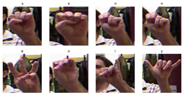
2. Visual data

plt.figure(figsize=(10, 5))  # The width of the figure is 10 and the height is 5

for images, labels in train_ds.take(1):
    for i in range(8):
        
        ax = plt.subplot(2, 4, i + 1)  

        plt.imshow(images[i].numpy().astype("uint8"))
        plt.title(class_names[labels[i]])
        
        plt.axis("off")

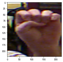
plt.imshow(images[1].numpy().astype("uint8"))

3. Recheck the data

for image_batch, labels_batch in train_ds:
    print(image_batch.shape)
    print(labels_batch.shape)
    break

(8, 224, 224, 3)
(8,)

• Image_batch is the tensor of the shape (8, 224, 224, 3). This is a batch of 8 pictures with shape of 240x240x3 (the last dimension refers to color channel RGB).
• Label_batch is the tensor of shape (8,), and these labels correspond to 8 pictures

4. Configure dataset

• shuffle(): scramble data. For a detailed description of this function, please refer to: https://zhuanlan.zhihu.com/p/42417456
• prefetch(): prefetch data and speed up operation. For details, please refer to my previous two articles, which are explained in them.
• cache(): cache data sets into memory to speed up operation

AUTOTUNE = tf.data.AUTOTUNE

train_ds = train_ds.cache().shuffle(1000).prefetch(buffer_size=AUTOTUNE)
val_ds = val_ds.cache().prefetch(buffer_size=AUTOTUNE)

If an error is reported, attributeerror: module 'tensorflow_ API. V2. Data 'has no attribute' autotune '. You can replace AUTOTUNE=tf.data.AUTOTUNE with autotune = tf.data.empirical.autotune

3, Introduction to Inception V3

For the introduction of inception series, see: https://baike.baidu.com/item/Inception%E7%BB%93%E6%9E%84 Personally, I think we only need to walk through the model (learn to build) at this stage. If necessary, we can go back and study it in detail later.

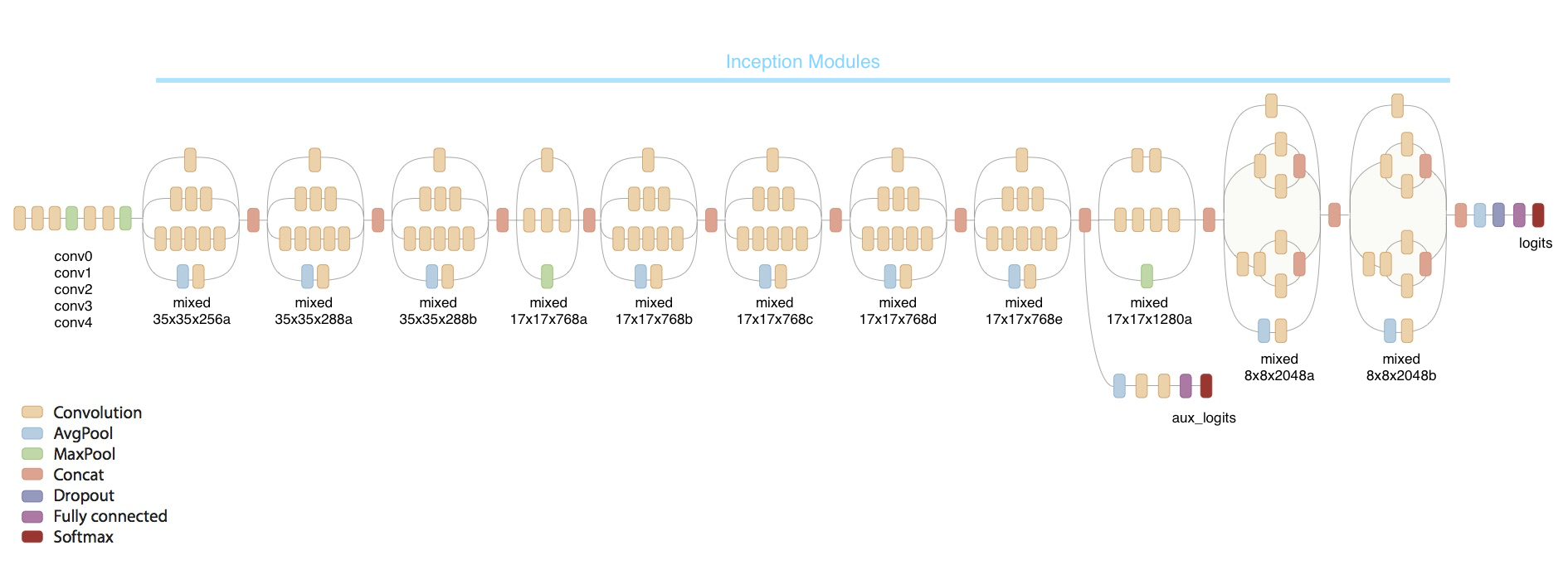
This model may be more complex than some models written before. First put a picture and feel it as a whole

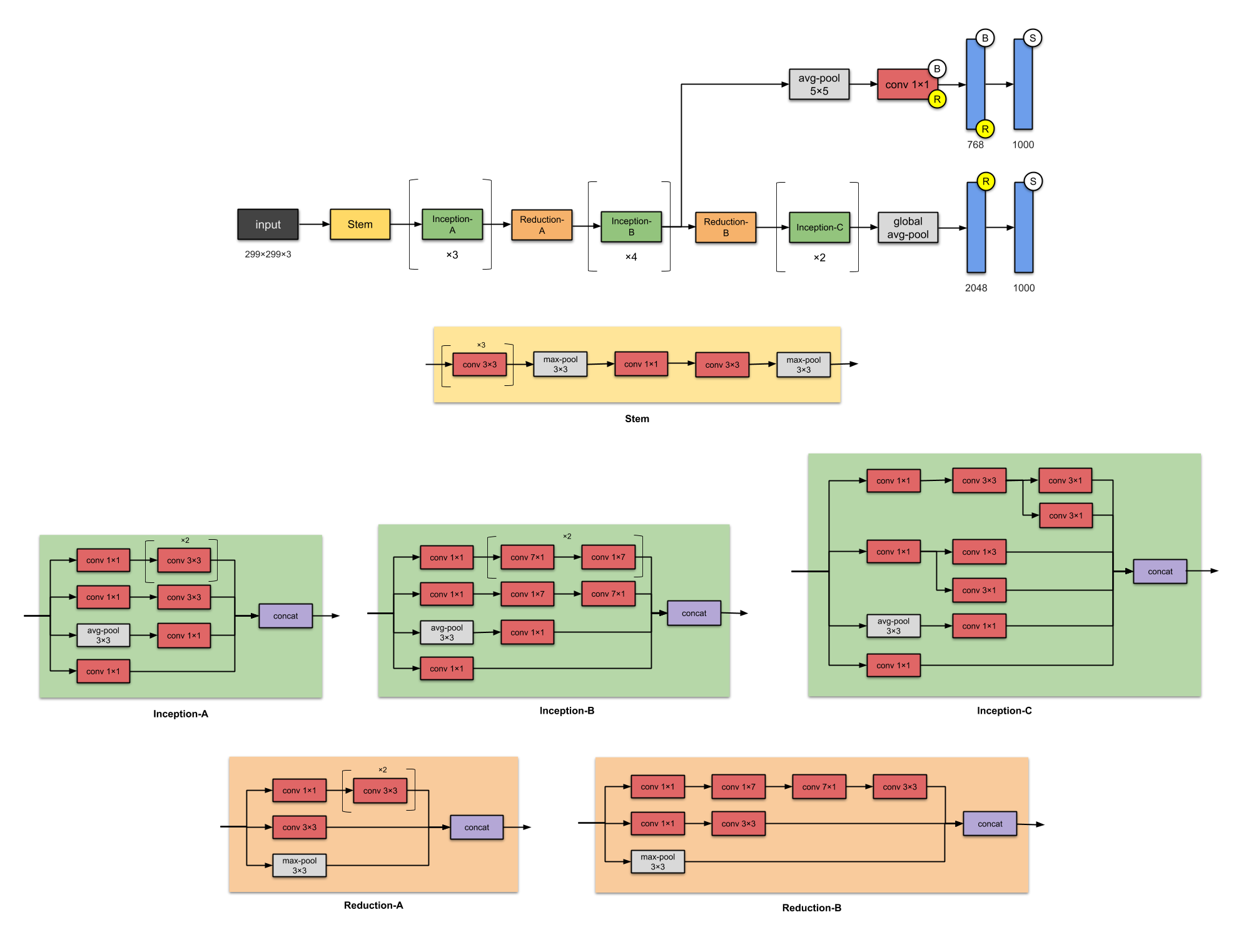
Another structural diagram, which is more detailed, can be clicked to view the larger one

The convolution calculation above is relatively simple. Students can refer to my article, ha: Calculation of convolution

4, Build Inception V3 network model

1. Build your own

The following is the focus of this article. You can try to build concept V3 according to the above figure. In this part, I mainly refer to the construction process of the official website and carry it out separately.

#=============================================================
#                  Inception V3 network                          
#=============================================================

from tensorflow.keras.models import Model
from tensorflow.keras        import layers
from tensorflow.keras.layers import Activation,Dense,Input,BatchNormalization,Conv2D,AveragePooling2D
from tensorflow.keras.layers import GlobalAveragePooling2D,MaxPooling2D


def conv2d_bn(x,filters,num_row,num_col,padding='same',strides=(1, 1),name=None):
    
    if name is not None:
        bn_name = name + '_bn'
        conv_name = name + '_conv'
    else:
        bn_name = None
        conv_name = None
        
    x = Conv2D(filters,(num_row, num_col),strides=strides,padding=padding,use_bias=False,name=conv_name)(x)
    x = BatchNormalization(scale=False, name=bn_name)(x)
    x = Activation('relu', name=name)(x)
    return x


def InceptionV3(input_shape=[224,224,3],classes=1000):

    img_input = Input(shape=input_shape)

    x = conv2d_bn(img_input, 32, 3, 3, strides=(2, 2), padding='valid')
    x = conv2d_bn(x, 32, 3, 3, padding='valid')
    x = conv2d_bn(x, 64, 3, 3)
    x = MaxPooling2D((3, 3), strides=(2, 2))(x)

    x = conv2d_bn(x,  80, 1, 1, padding='valid')
    x = conv2d_bn(x, 192, 3, 3, padding='valid')
    x = MaxPooling2D((3, 3), strides=(2, 2))(x)

    #================================#
    #         Block1 35x35
    #================================#
    # Block1 part1
    # 35 x 35 x 192 -> 35 x 35 x 256
    branch1x1 = conv2d_bn(x, 64, 1, 1)

    branch5x5 = conv2d_bn(x, 48, 1, 1)
    branch5x5 = conv2d_bn(branch5x5, 64, 5, 5)

    branch3x3dbl = conv2d_bn(x, 64, 1, 1)
    branch3x3dbl = conv2d_bn(branch3x3dbl, 96, 3, 3)
    branch3x3dbl = conv2d_bn(branch3x3dbl, 96, 3, 3)

    branch_pool = AveragePooling2D((3, 3), strides=(1, 1), padding='same')(x)
    branch_pool = conv2d_bn(branch_pool, 32, 1, 1)
    x = layers.concatenate([branch1x1, branch5x5, branch3x3dbl, branch_pool],axis=3,name='mixed0')

    # Block1 part2
    # 35 x 35 x 256 -> 35 x 35 x 288
    branch1x1 = conv2d_bn(x, 64, 1, 1)

    branch5x5 = conv2d_bn(x, 48, 1, 1)
    branch5x5 = conv2d_bn(branch5x5, 64, 5, 5)

    branch3x3dbl = conv2d_bn(x, 64, 1, 1)
    branch3x3dbl = conv2d_bn(branch3x3dbl, 96, 3, 3)
    branch3x3dbl = conv2d_bn(branch3x3dbl, 96, 3, 3)

    branch_pool = AveragePooling2D((3, 3), strides=(1, 1), padding='same')(x)
    branch_pool = conv2d_bn(branch_pool, 64, 1, 1)
    x = layers.concatenate([branch1x1, branch5x5, branch3x3dbl, branch_pool],axis=3,name='mixed1')

    # Block1 part3
    # 35 x 35 x 288 -> 35 x 35 x 288
    branch1x1 = conv2d_bn(x, 64, 1, 1)

    branch5x5 = conv2d_bn(x, 48, 1, 1)
    branch5x5 = conv2d_bn(branch5x5, 64, 5, 5)

    branch3x3dbl = conv2d_bn(x, 64, 1, 1)
    branch3x3dbl = conv2d_bn(branch3x3dbl, 96, 3, 3)
    branch3x3dbl = conv2d_bn(branch3x3dbl, 96, 3, 3)

    branch_pool = AveragePooling2D((3, 3), strides=(1, 1), padding='same')(x)
    branch_pool = conv2d_bn(branch_pool, 64, 1, 1)
    x = layers.concatenate([branch1x1, branch5x5, branch3x3dbl, branch_pool],axis=3,name='mixed2')

    #================================#
    #          Block2 17x17
    #================================#
    # Block2 part1
    # 35 x 35 x 288 -> 17 x 17 x 768
    branch3x3 = conv2d_bn(x, 384, 3, 3, strides=(2, 2), padding='valid')

    branch3x3dbl = conv2d_bn(x, 64, 1, 1)
    branch3x3dbl = conv2d_bn(branch3x3dbl, 96, 3, 3)
    branch3x3dbl = conv2d_bn(branch3x3dbl, 96, 3, 3, strides=(2, 2), padding='valid')

    branch_pool = MaxPooling2D((3, 3), strides=(2, 2))(x)
    x = layers.concatenate([branch3x3, branch3x3dbl, branch_pool], axis=3, name='mixed3')

    # Block2 part2
    # 17 x 17 x 768 -> 17 x 17 x 768
    branch1x1 = conv2d_bn(x, 192, 1, 1)

    branch7x7 = conv2d_bn(x, 128, 1, 1)
    branch7x7 = conv2d_bn(branch7x7, 128, 1, 7)
    branch7x7 = conv2d_bn(branch7x7, 192, 7, 1)

    branch7x7dbl = conv2d_bn(x, 128, 1, 1)
    branch7x7dbl = conv2d_bn(branch7x7dbl, 128, 7, 1)
    branch7x7dbl = conv2d_bn(branch7x7dbl, 128, 1, 7)
    branch7x7dbl = conv2d_bn(branch7x7dbl, 128, 7, 1)
    branch7x7dbl = conv2d_bn(branch7x7dbl, 192, 1, 7)

    branch_pool = AveragePooling2D((3, 3), strides=(1, 1), padding='same')(x)
    branch_pool = conv2d_bn(branch_pool, 192, 1, 1)
    
    x = layers.concatenate([branch1x1, branch7x7, branch7x7dbl, branch_pool],axis=3,name='mixed4')

    # Block2 part3 and part4
    # 17 x 17 x 768 -> 17 x 17 x 768 -> 17 x 17 x 768
    for i in range(2):
        branch1x1 = conv2d_bn(x, 192, 1, 1)

        branch7x7 = conv2d_bn(x, 160, 1, 1)
        branch7x7 = conv2d_bn(branch7x7, 160, 1, 7)
        branch7x7 = conv2d_bn(branch7x7, 192, 7, 1)

        branch7x7dbl = conv2d_bn(x, 160, 1, 1)
        branch7x7dbl = conv2d_bn(branch7x7dbl, 160, 7, 1)
        branch7x7dbl = conv2d_bn(branch7x7dbl, 160, 1, 7)
        branch7x7dbl = conv2d_bn(branch7x7dbl, 160, 7, 1)
        branch7x7dbl = conv2d_bn(branch7x7dbl, 192, 1, 7)

        branch_pool = AveragePooling2D(
            (3, 3), strides=(1, 1), padding='same')(x)
        branch_pool = conv2d_bn(branch_pool, 192, 1, 1)
        x = layers.concatenate([branch1x1, branch7x7, branch7x7dbl, branch_pool],axis=3,name='mixed' + str(5 + i))

    # Block2 part5
    # 17 x 17 x 768 -> 17 x 17 x 768
    branch1x1 = conv2d_bn(x, 192, 1, 1)

    branch7x7 = conv2d_bn(x, 192, 1, 1)
    branch7x7 = conv2d_bn(branch7x7, 192, 1, 7)
    branch7x7 = conv2d_bn(branch7x7, 192, 7, 1)

    branch7x7dbl = conv2d_bn(x, 192, 1, 1)
    branch7x7dbl = conv2d_bn(branch7x7dbl, 192, 7, 1)
    branch7x7dbl = conv2d_bn(branch7x7dbl, 192, 1, 7)
    branch7x7dbl = conv2d_bn(branch7x7dbl, 192, 7, 1)
    branch7x7dbl = conv2d_bn(branch7x7dbl, 192, 1, 7)

    branch_pool = AveragePooling2D((3, 3), strides=(1, 1), padding='same')(x)
    branch_pool = conv2d_bn(branch_pool, 192, 1, 1)
    x = layers.concatenate([branch1x1, branch7x7, branch7x7dbl, branch_pool],axis=3,name='mixed7')

    #================================#
    #         Block3 8x8
    #================================#
    # Block3 part1
    # 17 x 17 x 768 -> 8 x 8 x 1280
    branch3x3 = conv2d_bn(x, 192, 1, 1)
    branch3x3 = conv2d_bn(branch3x3, 320, 3, 3,strides=(2, 2), padding='valid')

    branch7x7x3 = conv2d_bn(x, 192, 1, 1)
    branch7x7x3 = conv2d_bn(branch7x7x3, 192, 1, 7)
    branch7x7x3 = conv2d_bn(branch7x7x3, 192, 7, 1)
    branch7x7x3 = conv2d_bn(branch7x7x3, 192, 3, 3, strides=(2, 2), padding='valid')

    branch_pool = MaxPooling2D((3, 3), strides=(2, 2))(x)
    x = layers.concatenate([branch3x3, branch7x7x3, branch_pool], axis=3, name='mixed8')

    # Block3 part2 part3
    # 8 x 8 x 1280 -> 8 x 8 x 2048 -> 8 x 8 x 2048
    for i in range(2):
        branch1x1 = conv2d_bn(x, 320, 1, 1)

        branch3x3 = conv2d_bn(x, 384, 1, 1)
        branch3x3_1 = conv2d_bn(branch3x3, 384, 1, 3)
        branch3x3_2 = conv2d_bn(branch3x3, 384, 3, 1)
        branch3x3 = layers.concatenate(
            [branch3x3_1, branch3x3_2], axis=3, name='mixed9_' + str(i))

        branch3x3dbl = conv2d_bn(x, 448, 1, 1)
        branch3x3dbl = conv2d_bn(branch3x3dbl, 384, 3, 3)
        branch3x3dbl_1 = conv2d_bn(branch3x3dbl, 384, 1, 3)
        branch3x3dbl_2 = conv2d_bn(branch3x3dbl, 384, 3, 1)
        branch3x3dbl = layers.concatenate([branch3x3dbl_1, branch3x3dbl_2], axis=3)

        branch_pool = AveragePooling2D((3, 3), strides=(1, 1), padding='same')(x)
        branch_pool = conv2d_bn(branch_pool, 192, 1, 1)
        x = layers.concatenate([branch1x1, branch3x3, branch3x3dbl, branch_pool],axis=3,name='mixed' + str(9 + i))
    
    # Full connection after average pooling.
    x = GlobalAveragePooling2D(name='avg_pool')(x)
    x = Dense(classes, activation='softmax', name='predictions')(x)

    inputs = img_input

    model = Model(inputs, x, name='inception_v3')

    return model

model = InceptionV3()
model.summary()

Model: "inception_v3"
__________________________________________________________________________________________________
Layer (type)                    Output Shape         Param #     Connected to                     
==================================================================================================
input_1 (InputLayer)            [(None, 224, 224, 3) 0                                            
__________________________________________________________________________________________________
conv2d (Conv2D)                 (None, 111, 111, 32) 864         input_1[0][0]                    
__________________________________________________________________________________________________
batch_normalization (BatchNorma (None, 111, 111, 32) 96          conv2d[0][0]                     
__________________________________________________________________________________________________
activation (Activation)         (None, 111, 111, 32) 0           batch_normalization[0][0]        
__________________________________________________________________________________________________
conv2d_1 (Conv2D)               (None, 109, 109, 32) 9216        activation[0][0]                 

......
__________________________________________________________________________________________________
avg_pool (GlobalAveragePooling2 (None, 2048)         0           mixed10[0][0]                    
__________________________________________________________________________________________________
predictions (Dense)             (None, 1000)         2049000     avg_pool[0][0]                   
==================================================================================================
Total params: 23,851,784
Trainable params: 23,817,352
Non-trainable params: 34,432
__________________________________________________________________________________________________

2. Official model

# import tensorflow as tf

# model_2 = tf.keras.applications.InceptionV3()
# model_2.summary()

5, Compile

Before preparing to train the model, you need to make some more settings. The following is added in the compilation step of the model:

• Loss function (loss): used to measure the accuracy of the model during training.
• optimizer: determines how the model updates based on the data it sees and its own loss function.
• metrics: used to monitor training and test steps. The following example uses the accuracy rate, that is, the ratio of images correctly classified.

# Setting the optimizer, I changed the learning rate here.
opt = tf.keras.optimizers.Adam(learning_rate=1e-5)

model.compile(optimizer=opt,
              loss='sparse_categorical_crossentropy',
              metrics=['accuracy'])

6, Training model

epochs = 10

history = model.fit(
    train_ds,
    validation_data=val_ds,
    epochs=epochs
)

Epoch 1/10
1255/1255 [==============================] - 130s 75ms/step - loss: 3.5247 - accuracy: 0.3366 - val_loss: 0.4606 - val_accuracy: 0.8776
Epoch 2/10
1255/1255 [==============================] - 68s 54ms/step - loss: 0.5796 - accuracy: 0.8711 - val_loss: 0.1501 - val_accuracy: 0.9530
Epoch 3/10
1255/1255 [==============================] - 68s 54ms/step - loss: 0.2236 - accuracy: 0.9589 - val_loss: 0.0639 - val_accuracy: 0.9825
Epoch 4/10
1255/1255 [==============================] - 69s 55ms/step - loss: 0.0803 - accuracy: 0.9917 - val_loss: 0.0403 - val_accuracy: 0.9884
Epoch 5/10
1255/1255 [==============================] - 71s 56ms/step - loss: 0.0333 - accuracy: 0.9989 - val_loss: 0.0239 - val_accuracy: 0.9928
Epoch 6/10
1255/1255 [==============================] - 70s 56ms/step - loss: 0.0165 - accuracy: 0.9992 - val_loss: 0.0168 - val_accuracy: 0.9944
Epoch 7/10
1255/1255 [==============================] - 70s 56ms/step - loss: 0.0076 - accuracy: 1.0000 - val_loss: 0.0160 - val_accuracy: 0.9944
Epoch 8/10
1255/1255 [==============================] - 70s 56ms/step - loss: 0.0041 - accuracy: 0.9999 - val_loss: 0.1108 - val_accuracy: 0.9737
Epoch 9/10
1255/1255 [==============================] - 70s 56ms/step - loss: 0.0358 - accuracy: 0.9919 - val_loss: 0.0312 - val_accuracy: 0.9888
Epoch 10/10
1255/1255 [==============================] - 69s 55ms/step - loss: 0.0111 - accuracy: 0.9985 - val_loss: 0.0068 - val_accuracy: 0.9980

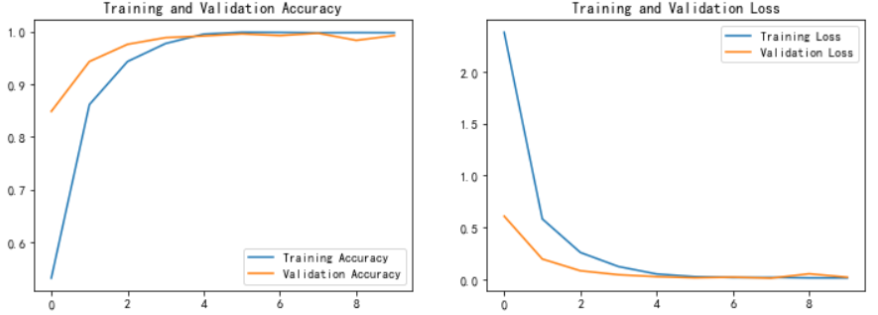
7, Model evaluation

acc = history.history['accuracy']
val_acc = history.history['val_accuracy']

loss = history.history['loss']
val_loss = history.history['val_loss']

epochs_range = range(epochs)

plt.figure(figsize=(12, 4))
plt.subplot(1, 2, 1)

plt.plot(epochs_range, acc, label='Training Accuracy')
plt.plot(epochs_range, val_acc, label='Validation Accuracy')
plt.legend(loc='lower right')
plt.title('Training and Validation Accuracy')

plt.subplot(1, 2, 2)
plt.plot(epochs_range, loss, label='Training Loss')
plt.plot(epochs_range, val_loss, label='Validation Loss')
plt.legend(loc='upper right')
plt.title('Training and Validation Loss')
plt.show()

8, Save and load model

This is the simplest method of model saving and loading

# Save model
model.save('model/13_model.h5')

# Loading model
new_model = keras.models.load_model('model/13_model.h5')

9, Forecast

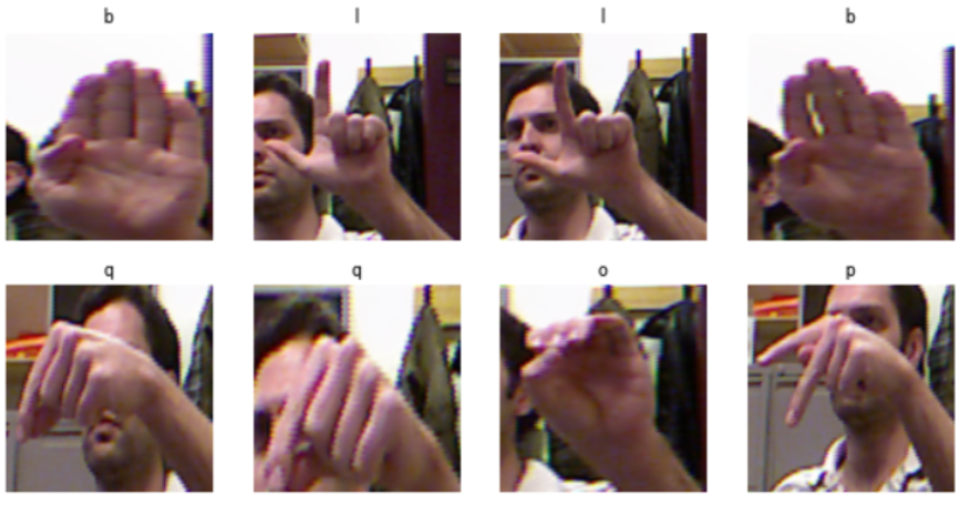
# Adopt loaded model (New)_ Model) to see the prediction results

plt.figure(figsize=(10, 5))  # The width of the figure is 10 and the height is 5

for images, labels in val_ds.take(1):
    for i in range(8):
        ax = plt.subplot(2, 4, i + 1)  
        
        # display picture
        plt.imshow(images[i].numpy().astype("uint8"))
        
        # You need to add a dimension to the picture
        img_array = tf.expand_dims(images[i], 0) 
        
        # Use the model to predict the characters in the picture
        predictions = new_model.predict(img_array)
        plt.title(class_names[np.argmax(predictions)])

        plt.axis("off")

Recommended reading

✨ This is too strong. I use it to identify traffic signs, and the accuracy is as high as 97.9%

✨ Convolutional neural network (AlexNet) hand-in-hand Teaching - 100 cases of deep learning | day 11

✨ Circular neural network (LSTM) realizes stock prediction - 100 cases of deep learning | day 10

✨ 100 cases of deep learning convolutional neural network (CNN) to realize mnist handwritten numeral recognition | day 1

🚀 From column: 100 cases of deep learning

Finally, I'll give you another copy to help you get the data structure brush notes of offer s from first-line manufacturers such as BAT. It was written by the bosses of Google and Alibaba. It is very useful for students who have weak algorithms or need to improve (extraction code: 9go2):

Leetcode notes of Google and Alibaba

And the 7K + open source e-books I sorted out, there is always one that can help you 💖( Extraction code: 4eg0)

7K + open source e-books

Unfinished ～

Continuous updates welcome likes 👍, Collection ⭐, follow 👀

• give the thumbs-up 👍: Praise gives me the motivation to continuously update
• Collection ⭐ Note: you can find articles at any time after collection
• follow 👀: Follow me to receive the latest articles for the first time