1, Introduction to firefly optimization algorithm (FA)
1 Introduction
There are many kinds of fireflies, mainly distributed in the tropics. Most fireflies produce rhythmic flashes in a short time. This flash is due to a chemical reaction of bioluminescence, and the flash pattern of fireflies varies from species to species. firefly algorithm (FA) is based on the flash behavior of fireflies. It is an intelligent random algorithm for global optimization problems, which was proposed by Yang Xin she (2009) [1]. Fireflies emit light through a chemical reaction in their lower abdomen, bioluminescence. This bioluminescence is an important part of the courtship ceremony of fireflies. It is also the main medium for male fireflies to communicate with female fireflies. The light can also be used to lure spouses or prey. At the same time, this flash also helps to protect the territory of fireflies and warn predators to stay away from their habitat. In FA, it is considered that all fireflies are hermaphroditic and attract each other regardless of gender. The algorithm is based on two key concepts: the intensity of light emitted and the degree of attraction between two fireflies.
2 behavior of natural fireflies
Natural fireflies show amazing flash behavior when looking for prey, attracting mates and protecting territory. Most fireflies live in tropical environment. Generally speaking, they produce cold light, such as green, yellow or light red. The attraction of a firefly depends on its light intensity. For any pair of fireflies, the brighter firefly will attract another firefly. Therefore, individuals with lower brightness move to brighter individuals, and the brightness of light decreases with the increase of distance. The flashing pattern of fireflies may vary from species to species. In some firefly species, females will use this phenomenon to hunt other species; Some fireflies show the behavior of synchronous flash in a large group of fireflies to attract prey. The female fireflies observe the flash emitted by the male fireflies from a stationary position. After finding an interesting flash, the female fireflies will respond and flash, and the courtship ceremony begins. Some female fireflies produce the flashing patterns of other fireflies to trap male fireflies and eat them.
3 firefly algorithm
The firefly algorithm simulates the natural phenomena of fireflies. Real fireflies naturally exhibit a discrete flicker pattern, and the firefly algorithm assumes that they are always glowing. In order to simulate the flickering behavior of fireflies, Yang Xin she proposed three rules (Yang, 2009):
(1) Assuming that all fireflies are hermaphroditic, one firefly may be attracted to any other firefly.
(2) The brightness of the firefly determines its attraction, and the brighter firefly attracts the darker firefly. If no firefly is brighter than the one under consideration, it will move randomly.
(3) The optimal value of the function is directly proportional to the brightness of the firefly.
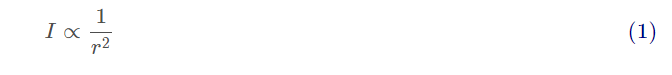
The light intensity (I) and the distance from the light source (r) obey the inverse square law. Therefore, due to the absorption of air, the light intensity (I) decreases with the increase of the distance from the light source. This phenomenon limits the visibility of fireflies to a very limited radius:
The main implementation steps of firefly algorithm are as follows:

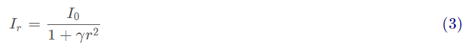
Where I0 is the light intensity (brightest) when the distance r=0, that is, its own brightness, which is related to the objective function value. The better the objective value, the brighter the brightness; γ Is the absorption coefficient. Because the fluorescence will gradually weaken with the increase of distance and the absorption of the media, the light intensity absorption coefficient can be set as a constant to reflect this characteristic; R is the distance between two fireflies. Monotone decreasing function is sometimes used, as shown in the following formula.
The second step is population initialization:

Where t represents algebra, xt represents the current position of the individual, β 0exp(- γ r2) is the degree of attraction, αε Is a random item. The next step is to calculate the attraction between Fireflies:
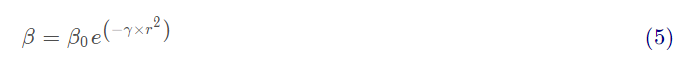
among β 0 represents the maximum attraction when r=0.
Next, low brightness fireflies move towards brighter Fireflies:

The last stage is to update the light intensity and sort all fireflies to determine the current best solution. The main steps of firefly algorithm are as follows.
Begin
	Basic parameters of initialization algorithm: set the number of fireflies n,Maximum attractionβ0,Light intensity absorption coefficientγ,Step factorα,Maximum number of iterations MaxGeneration Or search accuracyε;
	Initialization: randomly initialize the position of fireflies, and calculate the objective function value of fireflies as their maximum fluorescence brightness I0;
	t=1
	while(t<=MaxGeneration || accuracy>ε)
		Calculate the relative brightness of fireflies in the population I(Equation 2)And attractivenessβ(Equation 5), determining the moving direction of the firefly according to the relative brightness;
		Update the spatial position of fireflies and randomly move the fireflies in the best position (equation 6);
		Recalculate the brightness of the firefly according to the updated firefly position I0;
		t=t+1
	end while
	Output global extremum and optimal individual value.
end
Firefly algorithm is similar to particle swarm optimization (PSO) and bacterial foraging algorithm (BFA). In the position update equation, FA and PSO have two main components: one is deterministic and the other is stochastic. In FA, attraction is determined by two components: objective function and distance, while in BFA, attraction between bacteria also has two components: fitness and distance. When the firefly algorithm is implemented, the whole population (such as n) needs two inner loops and a specific iteration needs an outer loop (such as I). Therefore, the computational complexity of FA in the worst case is O(n2I).
2, Introduction to BP neural network
1 overview of BP neural network
BP (Back Propagation) neural network was proposed by the scientific research team headed by Rumelhart and McCelland in 1986. See their paper learning representations by Back Propagation errors published in Nature.
BP neural network is a multilayer feedforward network trained by error back propagation algorithm. It is one of the most widely used neural network models at present. BP network can learn and store a large number of input-output mode mapping relationships without revealing the mathematical equations describing this mapping relationship in advance. Its learning rule is to use the steepest descent method and continuously adjust the weight and threshold of the network through back propagation to minimize the sum of squares of the network error.
2 basic idea of BP algorithm
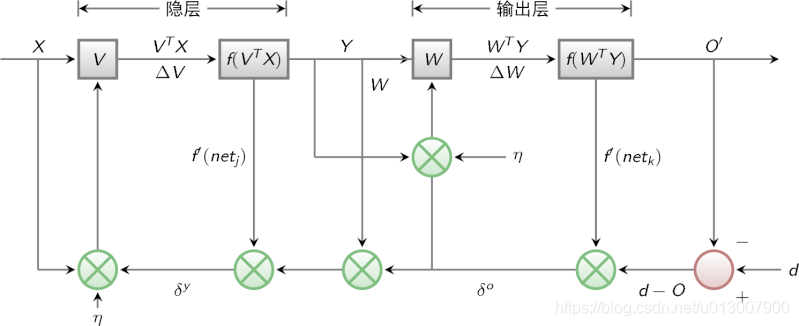
Last time we mentioned that multilayer perceptron encountered a bottleneck in how to obtain the weight of hidden layer. Since we can't get the weight of the hidden layer directly, can we indirectly adjust the weight of the hidden layer by getting the error between the output result and the expected output from the output layer? BP algorithm is designed with this idea. Its basic idea is that the learning process consists of two processes: forward propagation of signal and back propagation of error.
During forward propagation, the input samples are transmitted from the input layer, processed layer by layer by hidden layer, and then transmitted to the output layer. If the actual output of the output layer is inconsistent with the expected output (teacher signal), it will turn to the back propagation stage of error.
During back propagation, the output is transmitted back to the input layer layer by layer through the hidden layer in some form, and the error is allocated to all units of each layer, so as to obtain the error signal of each layer unit, which is used as the basis for correcting the weight of each unit. The specific processes of these two processes will be introduced later.
The signal flow diagram of BP algorithm is shown in the figure below
3 characteristic analysis of BP Network - three elements of BP
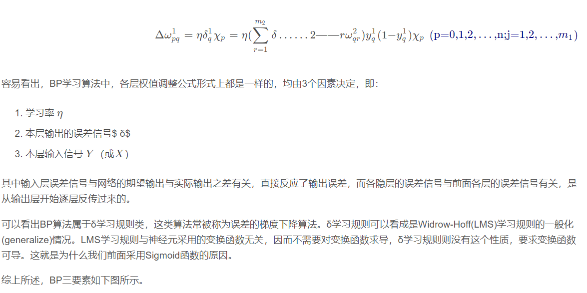
When we analyze an ANN, we usually start with its three elements, namely
1) Network topology;
2) Transfer function;
3) Learning algorithm.

The characteristics of each element together determine the functional characteristics of the ANN. Therefore, we also study BP network from these three elements.
3.1 topology of BP network
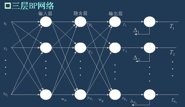
As I said last time, BP network is actually a multilayer perceptron, so its topology is the same as that of multilayer perceptron. Because the single hidden layer (three-layer) perceptron can solve simple nonlinear problems, it is most widely used. The topology of the three-layer perceptron is shown in the figure below.
The simplest three-layer BP:
3.2 transfer function of BP network
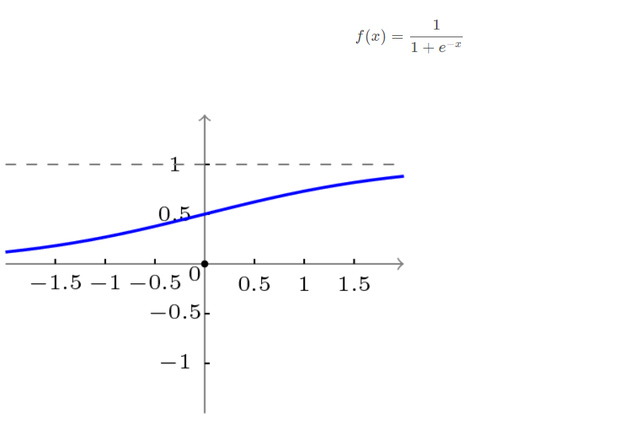
The transfer function used in BP network is a nonlinear transformation function - Sigmoid function (also known as S function). Its characteristic is that the function itself and its derivatives are continuous, so it is very convenient in processing. Why should we choose this function? I will give a further introduction when introducing the learning algorithm of BP network.
Unipolar S-type function curve is shown in the figure below.
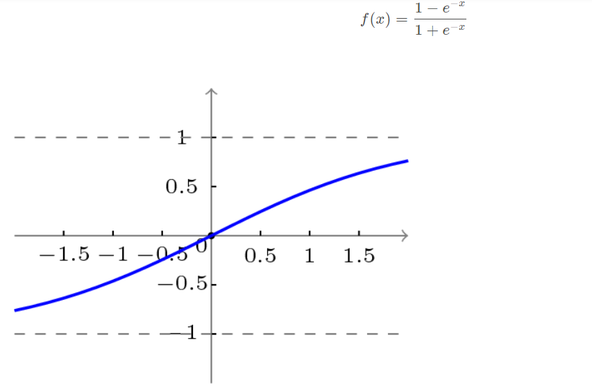
Bipolar S-type function curve is shown in the figure below.
3.3 learning algorithm of BP network
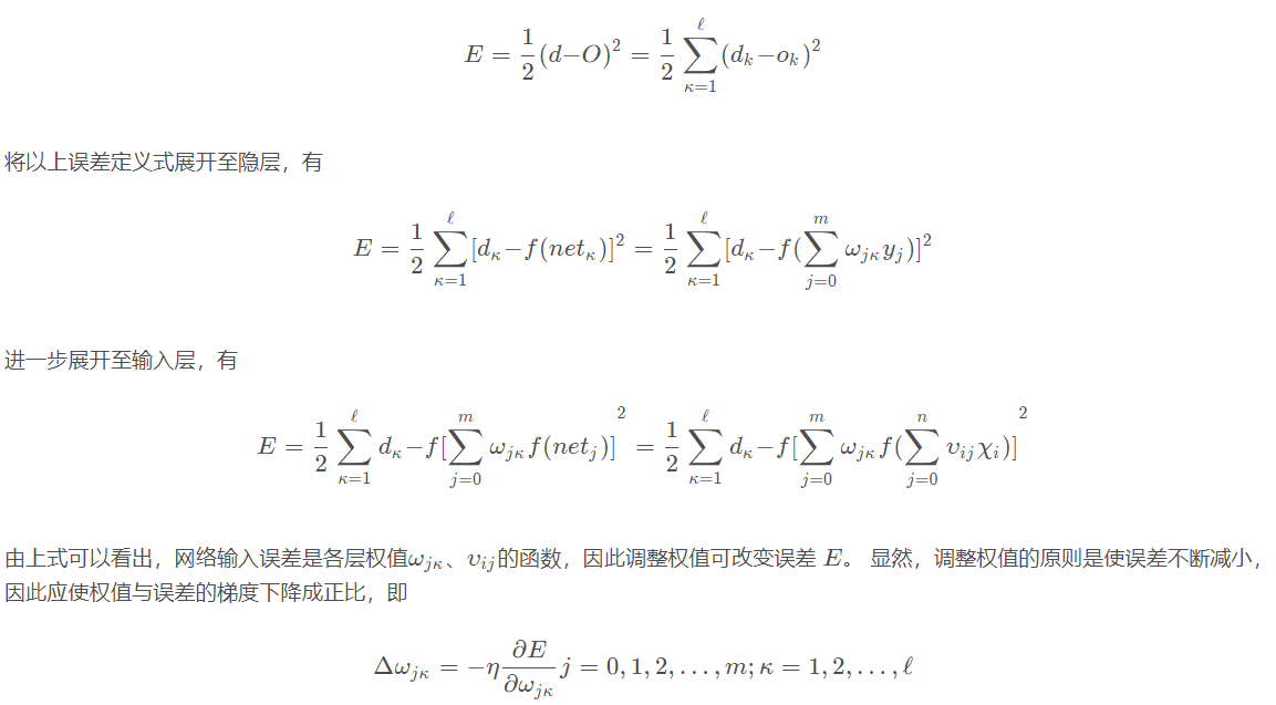
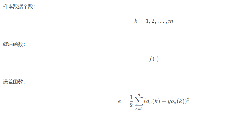
The learning algorithm of BP network is BP algorithm, also known as BP algorithm δ Algorithm (we will find many terms with multiple names in the learning process of ANN). Taking the three-layer perceptron as an example, when the network output is different from the expected output, there is an output error E, which is defined as follows

Next, we will introduce the specific process of BP network learning and training.
4 training decomposition of BP network
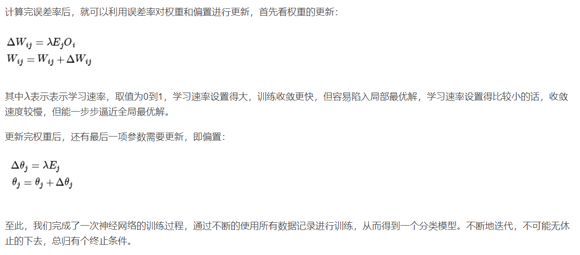
Training a BP neural network is actually adjusting the weight and bias of the network. The training process of BP neural network is divided into two parts:
Forward transmission, wave transmission output value layer by layer;
Reverse feedback, reverse layer by layer adjustment of weight and bias;
Let's look at forward transmission first.
Forward transmission (feed forward feedback)
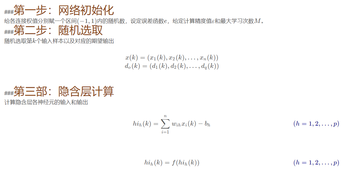
Before training the network, we need to initialize weights and offsets randomly, take a random real number of [− 1,1] [- 1,1] [− 1,1] for each weight, and a random real number of [0,1] [0,1] [0,1] for each offset, and then start forward transmission.
The training of neural network is completed by multiple iterations. Each iteration uses all records of the training set, while each training network uses only one record. The abstract description is as follows:
while Termination conditions not met:
    for record:dataset:
        trainModel(record)

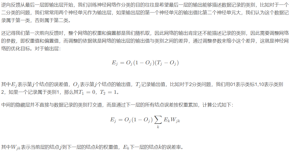
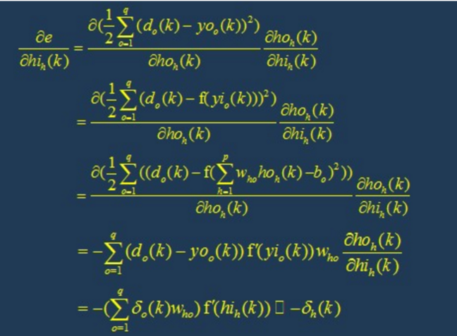
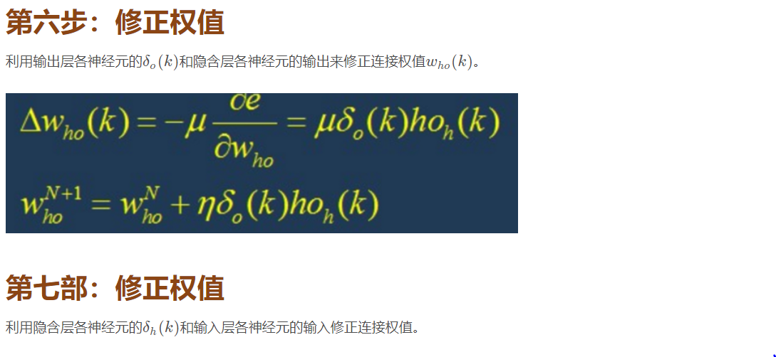
4.1 back propagation
4.2 training termination conditions
Each round of training uses all records of the data set, but when to stop, the stop conditions are as follows:
Set the maximum number of iterations, such as stopping training after 100 iterations with the dataset
Calculate the prediction accuracy of the training set on the network, and stop the training after reaching a certain threshold
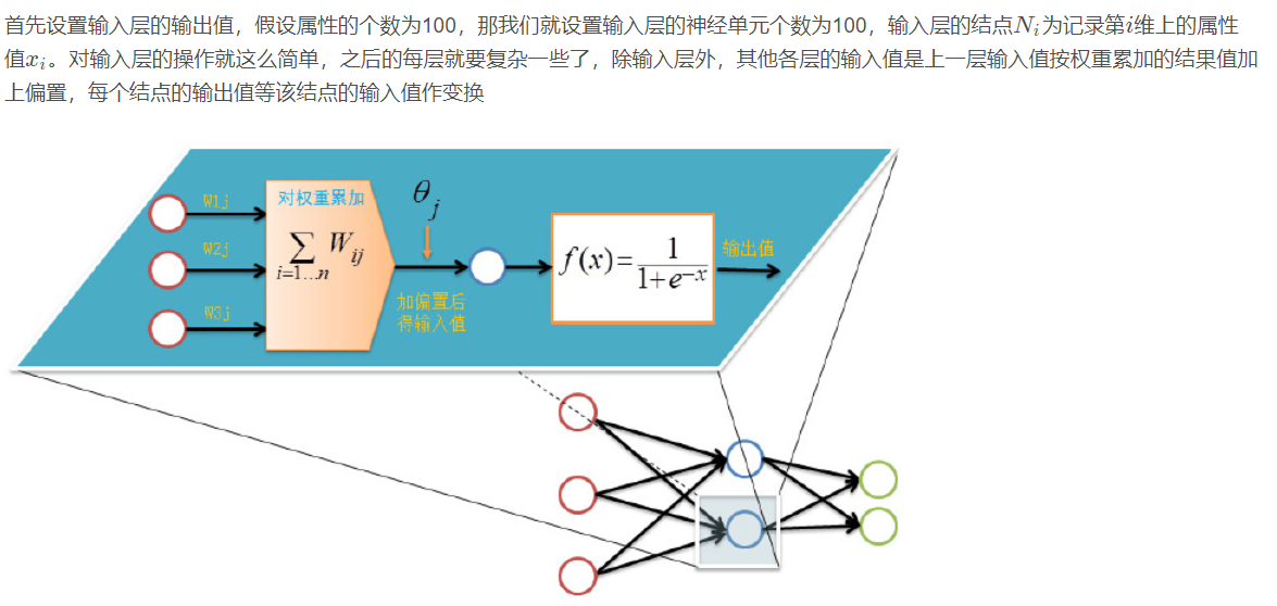
5. Specific process of BP network operation
5.1 network structure
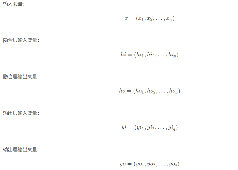
There are n nn neurons in the input layer, p pp neurons in the hidden layer and q qq neurons in the output layer.
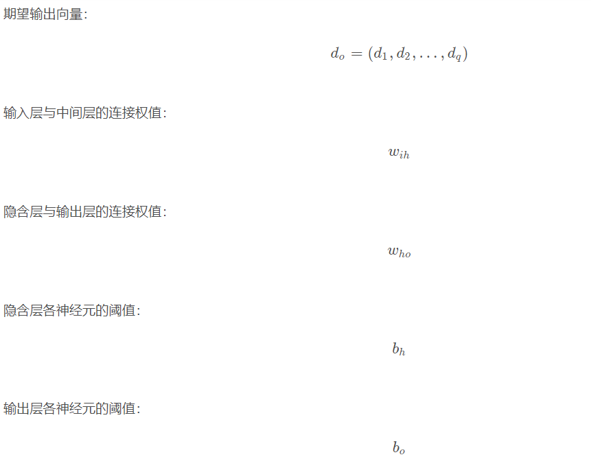
5.2 variable definition
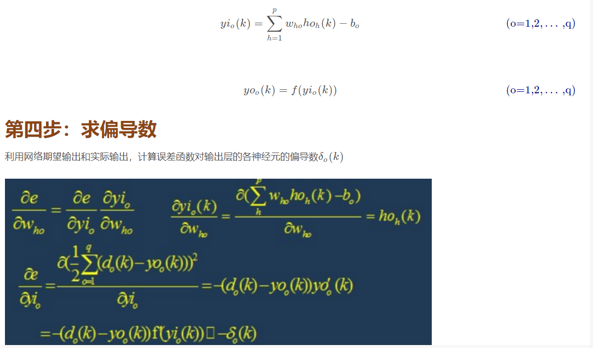
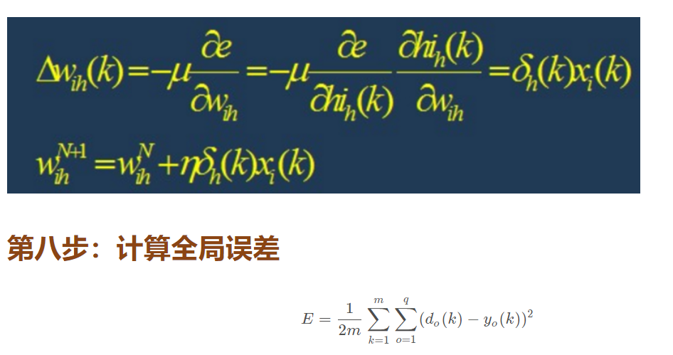
Step 9: judge the rationality of the model
Judge whether the network error meets the requirements.
When the error reaches the preset accuracy or the learning times are greater than the designed maximum times, the algorithm ends.
Otherwise, select the next learning sample and the corresponding output expectation, return to the third part and enter the next round of learning.
6 design of BP network
In the design of BP network, we should generally consider the number of layers of the network, the number of neurons and activation function in each layer, initial value and learning rate. The following are some selection principles.
6.1 network layers
Theory has proved that the network with deviation and at least one S-type hidden layer plus a linear output layer can approach any rational function. Increasing the number of layers can further reduce the error and improve the accuracy, but it is also the complexity of the network. In addition, the single-layer network with only nonlinear activation function can not be used to solve the problem, because the problems that can be solved with single-layer network can also be solved with adaptive linear network, and the operation speed of adaptive linear network is faster. For the problems that can only be solved with nonlinear function, the single-layer accuracy is not high enough, and only increasing the number of layers can achieve the desired results.
6.2 number of neurons in the hidden layer
The improvement of network training accuracy can be obtained by using a hidden layer and increasing the number of neurons, which is much simpler in structure than increasing the number of network layers. Generally speaking, we use accuracy and training network time to measure the quality of a neural network design:
(1) When the number of neurons is too small, the network can not learn well, the number of training iterations is relatively large, and the training accuracy is not high.
(2) When the number of neurons is too large, the more powerful the function of the network is, the higher the accuracy is, and the number of training iterations is also large, which may lead to over fitting.
Therefore, we get that the selection principle of the number of hidden layer neurons of neural network is: on the premise of solving the problem, add one or two neurons to speed up the decline of error.
6.3 selection of initial weight
Generally, the initial weight is a random number with a value between (− 1,1). In addition, after analyzing how the two-layer network trains a function, wedrow et al. Proposed a strategy to select the initial weight order as s √ r, where r is the number of inputs and S is the number of neurons in the first layer.
6.4 learning rate
The learning rate is generally 0.01 − 0.8. A large learning rate may lead to the instability of the system, but a small learning rate leads to too slow convergence and requires a long training time. For more complex networks, different learning rates may be required at different positions of the error surface. In order to reduce the training times and time to find the learning rate, a more appropriate method is to adopt the variable adaptive learning rate to make the network set different learning rates at different stages.
6.5 selection of expected error
In the process of designing the network, the expected error value should also determine an appropriate value after comparative training, which is determined relative to the required number of hidden layer nodes. Generally, two networks with different expected error values can be trained at the same time, and finally one of them can be determined by comprehensive factors.
7 limitations of BP network
BP network has the following problems:
(1) Long training time is required: This is mainly caused by the small learning rate, which can be improved by changing or adaptive learning rate.
(2) Completely unable to train: This is mainly reflected in the paralysis of the network. Generally, in order to avoid this situation, first, select a smaller initial weight, but use a smaller learning rate.
(3) Local minimum value: the gradient descent method adopted here may converge to the local minimum value, and better results may be obtained by using multi-layer network or more neurons.
8 improvement of BP network
The main goal of the improvement of P algorithm is to speed up the training speed and avoid falling into local minimum. The common improvement methods include the algorithm with momentum factor, adaptive learning rate, changing learning rate and action function contraction method. The basic idea of momentum factor method is to add a value proportional to the previous weight change to each weight change on the basis of back propagation, and generate a new weight change according to the back propagation method. The method of adaptive learning rate is aimed at some specific problems. The principle of the method of changing the learning rate is that if the sign of the objective function for the reciprocal of a weight is the same in several consecutive iterations, the learning rate of this weight will increase, on the contrary, if the sign is opposite, the learning rate will decrease. The contraction rule of the action function is to translate the action function, that is, add a constant.
3, Partial source code
%% Empty environment
clc
clear
%Read data
load data
z=data';
n=length(z);
for i=1:6;
sample(i,:)=z(i:i+n-6);
end
%Training data and prediction data
input_train=sample(1:5,1:1400);
output_train=sample(6,1:1400);
input_test=sample(1:5,1401:1483);
output_test=sample(6,1401:1483);
%Number of nodes
inputnum=5;
hiddennum=3;
outputnum=1;
%Build network
net=newff(inputn,outputn,hiddennum);
d=22;
%% The optimal initial threshold weight is given to the network prediction
% %Optimized by genetic algorithm BP Network value prediction
dennum+hiddennum+hiddennum*outputnum);
B2=x(inputnum*hiddennum+hiddennum+hiddennum*outputnum+1:inputnum*hiddennum+hiddennum+hiddennum*outputnum+outputnum);
net.iw{1,1}=reshape(w1,hiddennum,inputnum);
net.lw{2,1}=reshape(w2,outputnum,hiddennum);
net.b{1}=reshape(B1,hiddennum,1);
net.b{2}=B2;
%% BP Network training
%Network evolution parameters
net.trainParam.epochs=100;
net.trainParam.lr=0.1;
%net.trainParam.goal=0.00001;
%Network training
[net,per2]=train(net,inputn,outputn);
%% BP Network prediction
%data normalization
inputn_test=mapminmax('apply',input_test,inputps);
an=sim(net,inputn_test);
test_simu=mapminmax('reverse',an,outputps);
error=test_simu-output_test;
E=mean(abs(error./output_test))
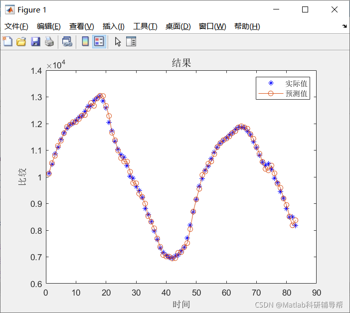
plot(output_test,'b*')
hold on;
plot(test_simu,'-o')
title('result','fontsize',12)
legend('actual value','Estimate')
xlabel('time')
ylabel('compare')
%% Cost or Objective function
function [nbest,fbest,NumEval]=ffa_mincon(u0,Lb,Ub,para,inputnum,hiddennum,outputnum,net,inputn,outputn) % para=[20 500 0.5 0.2 1];
% Check input parameters (otherwise set as default values)
if nargin<5, para=[20 50 0.25 0.20 1]; end
if nargin<4, Ub=[]; end
if nargin<3, Lb=[]; end
if nargin<2,
disp('Usuage: FA_mincon(@cost,u0,Lb,Ub,para)');
end
% n=number of fireflies
% MaxGeneration=number of pseudo time steps
% ------------------------------------------------
% alpha=0.25; % Randomness 0--1 (highly random)
% betamn=0.20; % minimum value of beta
% gamma=1; % Absorption coefficient
% ------------------------------------------------
n=para(1);
MaxGeneration=para(2); %MaxGeneration
alpha=para(3);
betamin=para(4);
gamma=para(5);
NumEval=n*MaxGeneration;
% Check if the upper bound & lower bound are the same size
if length(Lb) ~=length(Ub),
disp('Simple bounds/limits are improper!');
return
end
% Calcualte dimension
d=length(u0); %
% Initial values of an array
zn=ones(n,1)*10^100;
% ------------------------------------------------
% generating the initial locations of n fireflies
[ns,Lightn]=init_ffa(n,d,Lb,Ub,u0); %
% Iterations or pseudo time marching
for k=1:MaxGeneration, %%%%% start iterations
% This line of reducing alpha is optional
alpha=alpha_new(alpha,MaxGeneration);
% Evaluate new solutions (for all n fireflies)
for i=1:n,
zn(i)=fun(ns(i,:),inputnum,hiddennum,outputnum,net,inputn,outputn);
Lightn(i)=zn(i);
end
function error = fun(x,inputnum,hiddennum,outputnum,net,inputn,outputn)
%This function is used to calculate the fitness value
%x input individual
%inputnum input Enter the number of layer nodes
%outputnum input Number of hidden layer nodes
%net input network
%inputn input Training input data
%outputn input Training output data
%error output Individual fitness value
%extract
w1=x(1:inputnum*hiddennum);%Ten weights
B1=x(inputnum*hiddennum+1:inputnum*hiddennum+hiddennum);%Five thresholds
w2=x(inputnum*hiddennum+hiddennum+1:inputnum*hiddennum+hiddennum+hiddennum*outputnum);%Five weights
B2=x(inputnum*hiddennum+hiddennum+hiddennum*outputnum+1:inputnum*hiddennum+hiddennum+hiddennum*outputnum+outputnum);%A threshold
%Network evolution parameters
net.trainParam.epochs=20;
net.trainParam.lr=0.1;
net.trainParam.goal=0.00001;
net.trainParam.show=100;
net.trainParam.showWindow=false;
%Network weight assignment
net.iw{1,1}=reshape(w1,hiddennum,inputnum);
net.lw{2,1}=reshape(w2,outputnum,hiddennum);
net.b{1}=reshape(B1,hiddennum,1);
net.b{2}=B2;
%Should be net It's a structure, and then the first one net.IW{1,1}Refers to the weight input from the first layer to the hidden layer,
%The first 1 represents the hidden layer, in sharp contrast to the second line of code: net.IW{2,1}That is, the weight from the input vector of the first hidden layer to the output layer,
%2 in this represents the output layer. After sorting out these, we can see that it is obvious: the right side of the first assignment is the first one w1 Number of hidden layers for matrix deformation*Enter the number of layers.
%The second is from the hidden layer to the output layer, where W1,W2 Are weight matrices. The last line is the threshold assignment of the first layer (represented by 1).
%Network training
net=train(net,inputn,outputn);
an=sim(net,inputn);
error=sum(abs(an-outputn));
4, Operation results
5, matlab version and references
1 matlab version
2014a
2 references
[1] Baoziyang, Yu Jizhou, Yang Shan. Intelligent optimization algorithm and its MATLAB example (2nd Edition) [M]. Electronic Industry Press, 2016
[2] Zhang Yan, Wu Shuigen. MATLAB optimization algorithm source code [M]. Tsinghua University Press, 2017
[3]Firefly Algorithm (FA) of swarm intelligence optimization algorithm