Zero basis entry financial risk control - loan default forecast
1, Competition data
The task of the competition is to predict whether users default on their loans. The data set can be seen and downloaded after registration. The data comes from the loan records of A credit platform. The total amount of data exceeds 120w, including 47 columns of variable information, of which 15 columns are anonymous variables. In order to ensure the fairness of the competition, 800000 will be selected as the training set, 200000 as the test set A and 200000 as the test set B. at the same time, the information such as employmentTitle, purpose, postCode and title will be desensitized.
Data can be obtained in Alibaba cloud learning contest.
- Field table
| id | Field | Description |
|---|---|---|
| 1 | id | Unique letter of credit identifier assigned to the loan list |
| 2 | loanAmnt | Loan amount |
| 3 | term | Loan term (year) |
| 4 | interestRate | lending rate |
| 5 | installment | Installment amount |
| 6 | grade | Loan grade |
| 7 | subGrade | Sub level of loan grade |
| 8 | employmentTitle | Employment title |
| 9 | employmentLength | Years of employment (years) |
| 10 | homeOwnership | The ownership status of the house provided by the borrower at the time of registration |
| 11 | annualIncome | annual income |
| 12 | verificationStatus | Verification status |
| 13 | issueDate | Month of loan issuance |
| 14 | purpose | Loan purpose category of the borrower at the time of loan application |
| 15 | postCode | The first three digits of the postal code provided by the borrower in the loan application |
| 16 | regionCode | Area code |
| 17 | dti | Debt to income ratio |
| 18 | delinquency_2years | Number of events of default in the borrower's credit file overdue for more than 30 days in the past two years |
| 19 | ficoRangeLow | The lower limit of the borrower's fico at the time of loan issuance |
| 20 | ficoRangeHigh | The upper limit of the borrower's fico at the time of loan issuance |
| 21 | openAcc | The number of open credit lines in the borrower's credit file |
| 22 | pubRec | Number of derogatory public records |
| 23 | pubRecBankruptcies | Number of public records cleared |
| 24 | revolBal | Total credit turnover balance |
| 25 | revolUtil | RCF utilization, or the amount of credit used by the borrower relative to all available RCFs |
| 26 | totalAcc | Total current credit limit in the borrower's credit file |
| 27 | initialListStatus | Initial list status of loans |
| 28 | applicationType | Indicates whether the loan is an individual application or a joint application with two co borrowers |
| 29 | earliesCreditLine | The month in which the borrower first reported the opening of the credit line |
| 30 | title | Name of loan provided by the borrower |
| 31 | policyCode | Publicly available policies_ Code = 1 new product not publicly available policy_ Code = 2 |
| 32 | n-series anonymous feature | Anonymous feature n0-n14, which is the processing of counting features for some lender behaviors |
2, Evaluation criteria
The submitted result is the probability that each test sample is 1, that is, the probability that y is 1. The evaluation method is AUC to evaluate the effect of the model (the larger the better).
3, Code demonstration
- Note: the following operation results are part of the diagram.
- Environment: library used in this case
- pandas 1.3.2
- matplotlib 3.4.3
- seaborn 0.11.2
- numpy 1.21.2
- scipy 1.4.1
- scikit-learn 0.24.2
- Using the jupyter notebook
1. Data analysis and processing
1.1.0 import related libraries
import pandas as pd
import matplotlib.pyplot as plt
import seaborn as sns
import numpy as np
from scipy import stats
import matplotlib as mpl
#Show all columns
pd.set_option('display.max_columns',None)
# Warning handling
import warnings
warnings.filterwarnings('ignore')
%matplotlib inline
1.1.1 data preprocessing
df_train = pd.read_csv('train.csv')
df_test = pd.read_csv('testA.csv')
df_train.shape, df_test.shape

df_train['train_test'] = 'train'
df_test['train_test'] = 'test'
Merge training set and test set
df = df_train.append(df_test)
df.reset_index(inplace=True)
df.drop('index',inplace=True,axis=1)
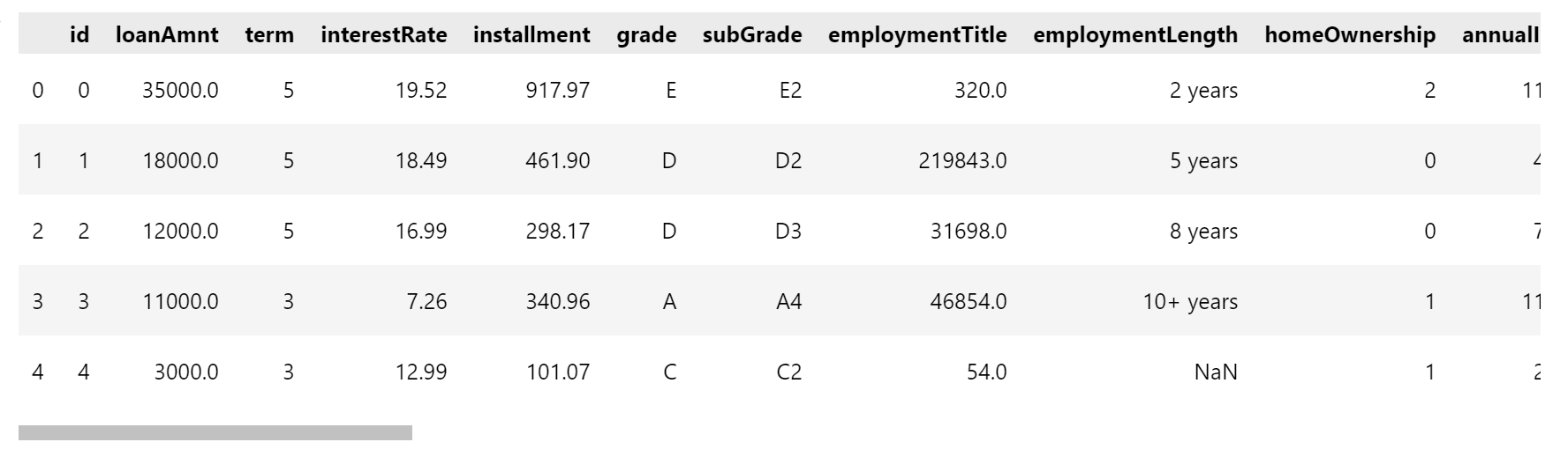
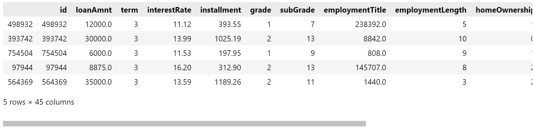
display(df.head())
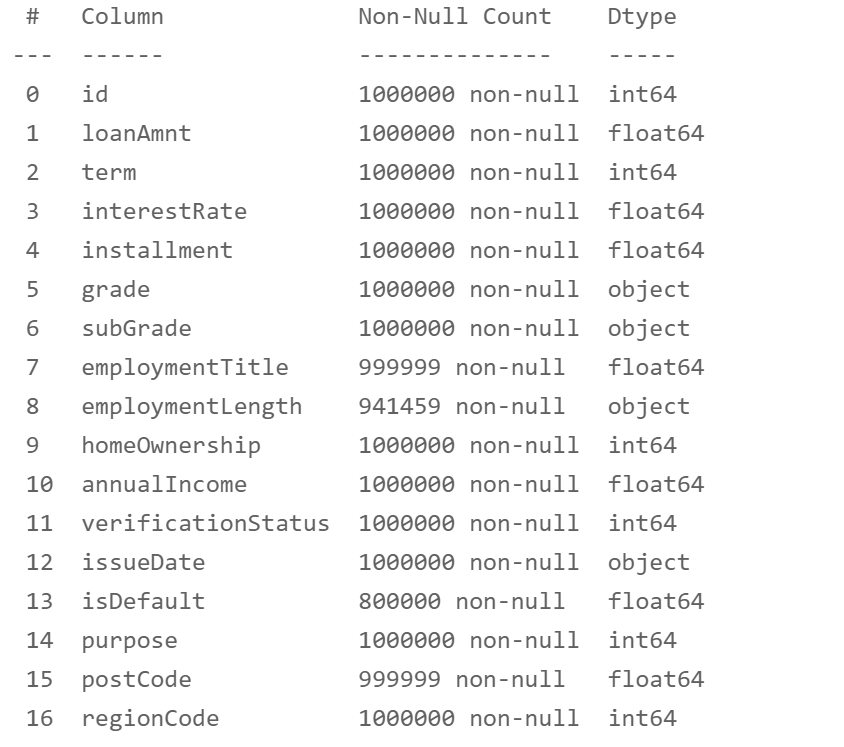
df.info()
Missing value processing
# Column names to process
is_na_cols = [
    'employmentTitle', 'employmentLength', 'postCode', 'dti', 'pubRecBankruptcies',
    'revolUtil', 'title',] + [f'n{i}' for i in range(15)]
Fill the missing values with modes
# Fill the missing values with modes
for i in range(len(is_na_cols)):
most_num = df[is_na_cols[i]].value_counts().index[0]
df[is_na_cols[i]] = df[is_na_cols[i]].fillna(most_num)
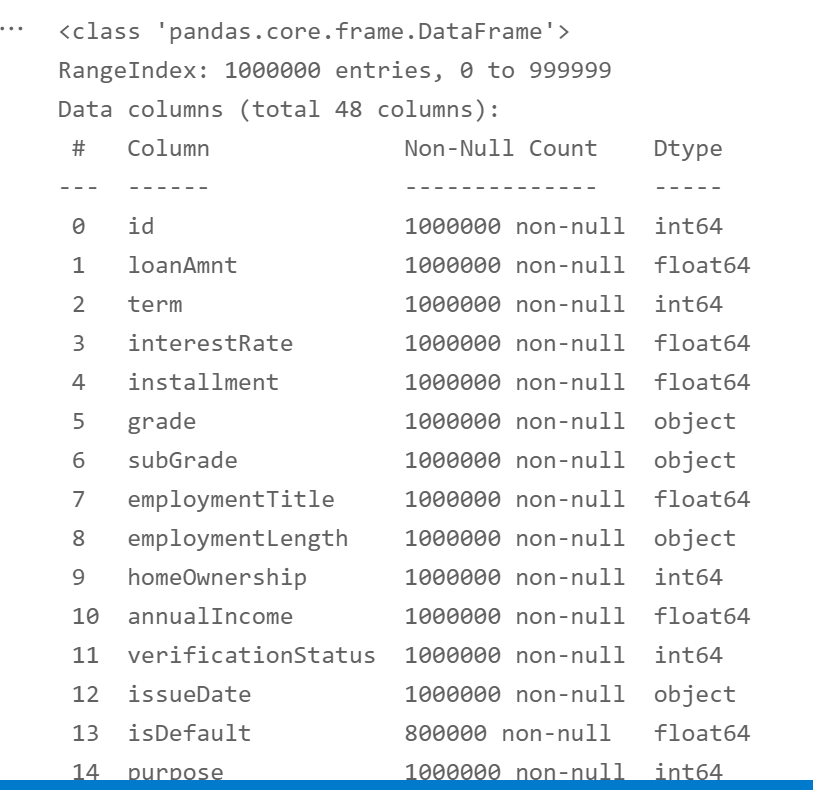
df.info()
Separate training set and test set
df_train = df[df['train_test'] == 'train']
df_test = df[df['train_test'] == 'test']
del df_train['train_test']
del df_test['train_test']
df_train.shape, df_test.shape

Delete forecast target for test set
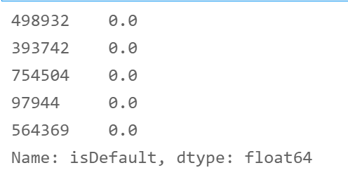
del df_test['isDefault']
1.1.2 processing and analysis of numerical and non numerical variables
# Non numerical type
non_numeric_cols = [
'grade', 'subGrade', 'employmentLength', 'issueDate', 'earliesCreditLine'
]
# Numerical type
numeric_cols = [
x for x in df_test.columns if x not in non_numeric_cols + ['isDefault']
]
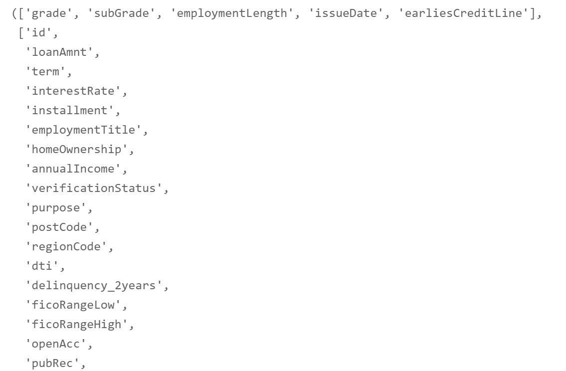
non_numeric_cols, numeric_cols
1.1.3 numerical_cols test set and training set distribution
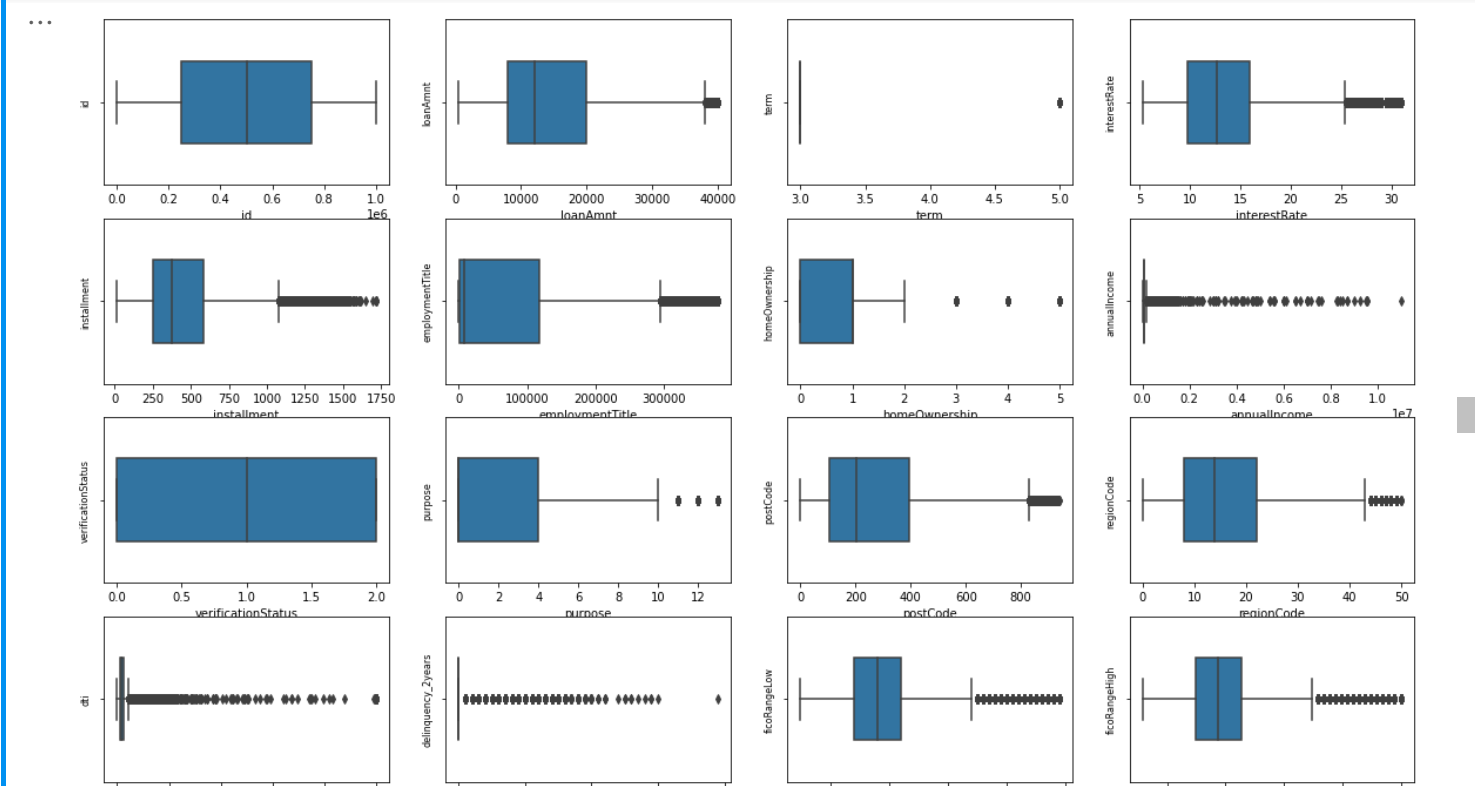
Draw a box chart to see which column names are continuous and discontinuous variables
# Draw box diagram
column = numeric_cols # List header
fig = plt.figure(figsize=(20, 40))  # Specifies the width and height of the drawing object
for i in range(len(column)):
    plt.subplot(13, 4, i + 1)  # 13 row 3 column subgraph
    sns.boxplot(df[column[i]], orient="v", width=0.5)  # Box diagram
    plt.ylabel(column[i], fontsize=8)
plt.show()
1.1.4 take out the numerical continuity variable and check the data distribution
continuous_cols = [
    'id', 'loanAmnt', 'interestRate', 'installment', 'employmentTitle', 'homeOwnership',
    'annualIncome', 'purpose', 'postCode', 'regionCode', 'dti', 'delinquency_2years',
    'ficoRangeLow', 'ficoRangeHigh', 'openAcc', 'pubRec', 'revolBal', 'revolUtil','totalAcc',
    'title', 'n14'
] + [f'n{i}' for i in range(11)]
non_continuous_cols = [
    x for x in numeric_cols if x not in continuous_cols
]
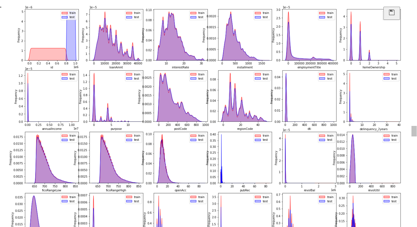
Visualize the Zhengtai distribution to see whether the data of the test set and the training set are the same and can be retained. If the gap will affect the prediction results, it will be removed.
dist_cols = 6
dist_rows = len(df_test[continuous_cols].columns)
plt.figure(figsize=(4*dist_cols,4*dist_rows))

i=1
for col in df_test[continuous_cols].columns:
    ax=plt.subplot(dist_rows,dist_cols,i)
    ax = sns.kdeplot(df_train[continuous_cols][col], color="Red", shade=True)
    ax = sns.kdeplot(df_test[continuous_cols][col], color="Blue", shade=True)
    ax.set_xlabel(col)
    ax.set_ylabel("Frequency")
    ax = ax.legend(["train","test"])

    i+=1
plt.show()
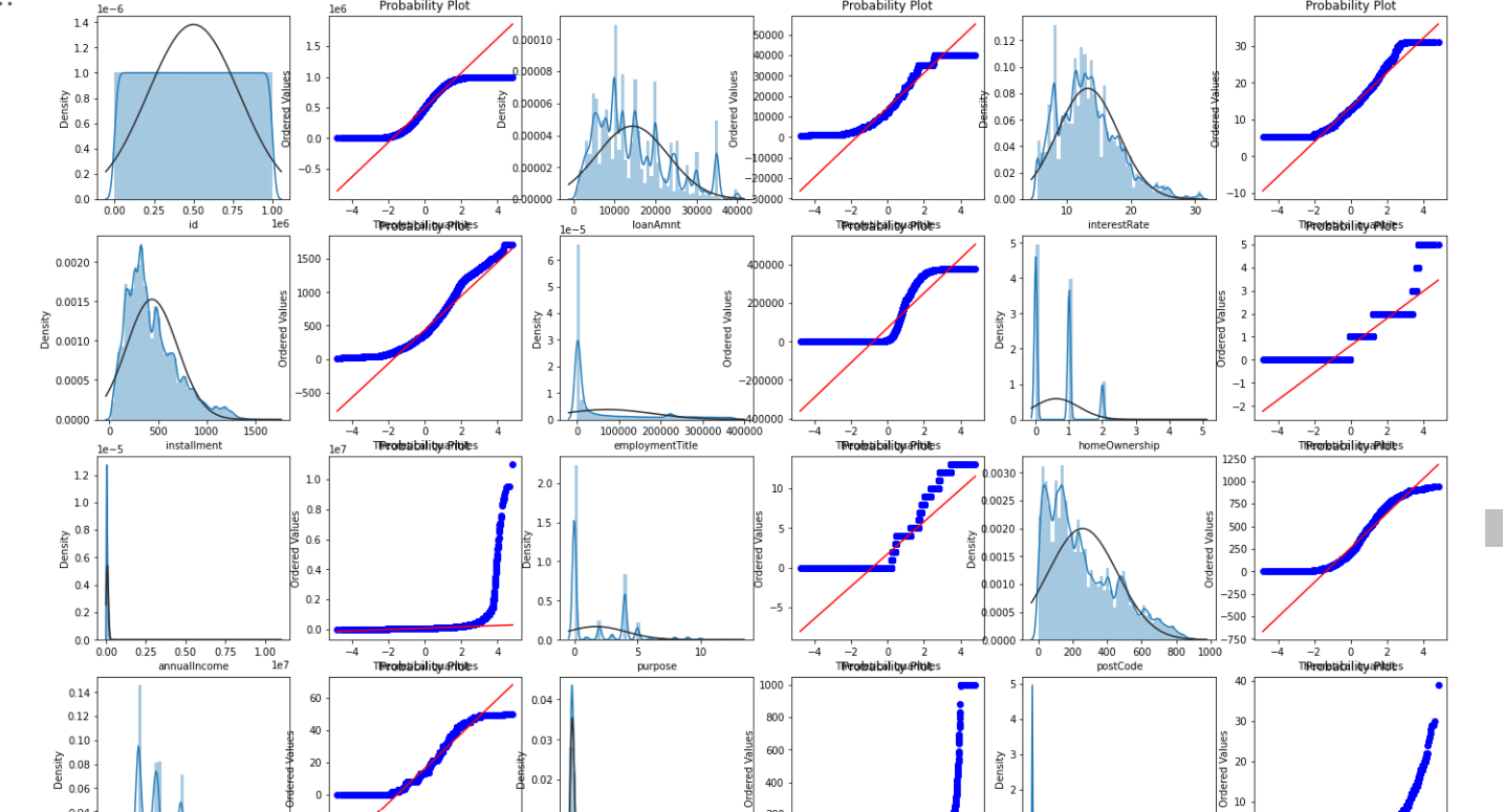
Draw QQ diagram and normal distribution diagram
- QQ chart: the closer the curve is to the straight line, the closer it is to the normal distribution, and the better the prediction effect is.
train_cols = 6
train_rows = len(df[continuous_cols].columns)
plt.figure(figsize=(4*train_cols,4*train_rows))

i=0
for col in df[continuous_cols].columns:
    i+=1
    ax=plt.subplot(train_rows,train_cols,i)
    sns.distplot(df[continuous_cols][col],fit=stats.norm)
    i+=1
    ax=plt.subplot(train_rows,train_cols,i)
    res = stats.probplot(df[continuous_cols][col], plot=plt)
plt.show()
The data distribution of training set and test set is almost the same, and they can be integrated for processing
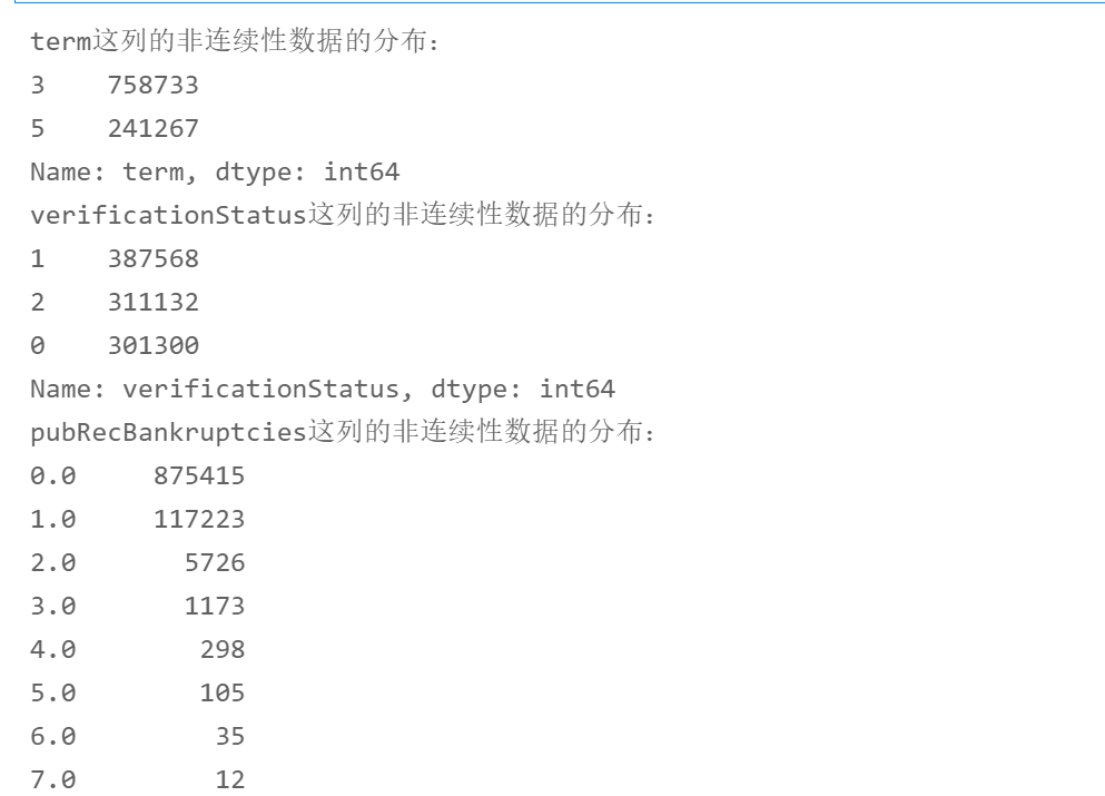
1.1.5 viewing numerical discontinuous data distribution
for i in range(len(non_continuous_cols)):
    print("%s Distribution of discontinuous data in this column:"%non_continuous_cols[i])
    print(df[non_continuous_cols[i]].value_counts())
1.1.6 viewing non numeric data distribution
for i in range(len(non_numeric_cols)):
    print("%s This is the distribution of non numeric data:\n"%non_numeric_cols[i])
    print(df[non_numeric_cols[i]].value_counts())

2. Characteristic Engineering
2.1.1 numerical discontinuous data processing
- policyCode field
df['policyCode'].describe()
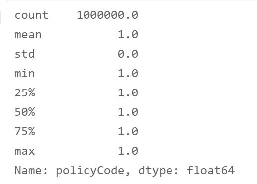
# The field has only one value. No need
df.drop('policyCode',axis=1,inplace=True)
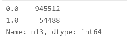
- n13 field
df['n13'] = df['n13'].apply(lambda x: 1 if x not in [0] else x)
df['n13'].value_counts()
2.1.2 non numerical data
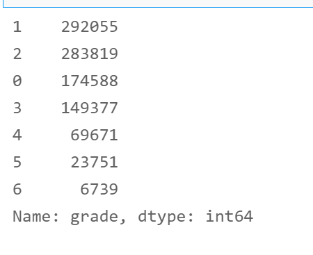
- grade field
# Non numeric coding
from sklearn.preprocessing import LabelEncoder
le = LabelEncoder()
df['grade'] = le.fit_transform(df['grade'])
df['grade'].value_counts()
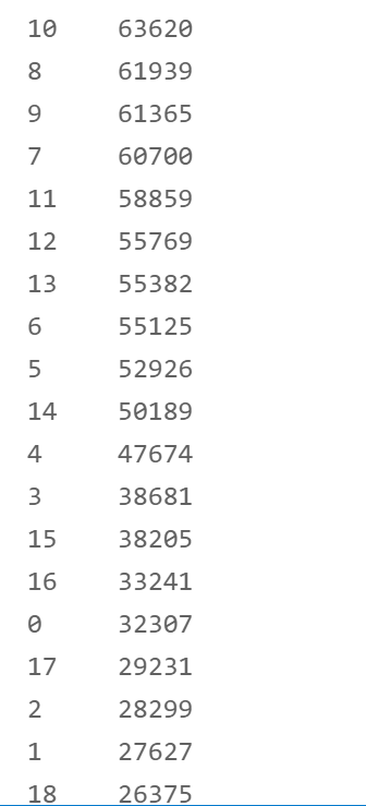
2. subGrade field
from sklearn.preprocessing import LabelEncoder
le = LabelEncoder()
df['subGrade'] = le.fit_transform(df['subGrade'])
df['subGrade'].value_counts()
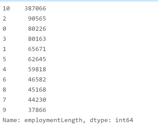
3. employmentLength field
# Construct coding function
def encoder(x):
    if x[:-5] == '10+ ':
        return 10
    elif x[:-5] == '< 1':
        return 0
    else:
        return int(x[0])
df['employmentLength'] = df['employmentLength'].apply(encoder)
df['employmentLength'].value_counts()
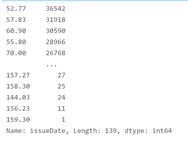
4. issueDate field
- It's ok to calculate how many months from now
from datetime import datetime
def encoder1(x):
    x = str(x)
    now = datetime.strptime('2020-07-01','%Y-%m-%d')
    past = datetime.strptime(x,'%Y-%m-%d')
    period = now - past
    period = period.days
    return round(period / 30, 2)
df['issueDate'] = df['issueDate'].apply(encoder1)
df['issueDate'].value_counts()
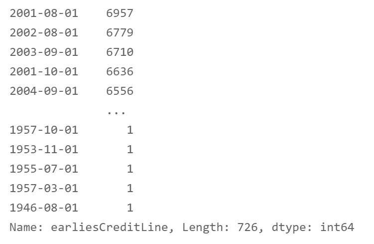
5. earliesCreditLine field
def encoder2(x):
    if x[:3] == 'Jan':
        return x[-4:] + '-' + '01-01'
    if x[:3] == 'Feb':
        return x[-4:] + '-' + '02-01'
    if x[:3] == 'Mar':
        return x[-4:] + '-' + '03-01'
    if x[:3] == 'Apr':
        return x[-4:] + '-' + '04-01'
    if x[:3] == 'May':
        return x[-4:] + '-' + '05-01'
    if x[:3] == 'Jun':
        return x[-4:] + '-' + '06-01'
    if x[:3] == 'Jul':
        return x[-4:] + '-' + '07-01'
    if x[:3] == 'Aug':
        return x[-4:] + '-' + '08-01'
    if x[:3] == 'Sep':
        return x[-4:] + '-' + '09-01'
    if x[:3] == 'Oct':
        return x[-4:] + '-' + '10-01'
    if x[:3] == 'Nov':
        return x[-4:] + '-' + '11-01'
    if x[:3] == 'Dec':
        return x[-4:] + '-' + '12-01'
df['earliesCreditLine'] = df['earliesCreditLine'].apply(encoder2)
df['earliesCreditLine'].value_counts()
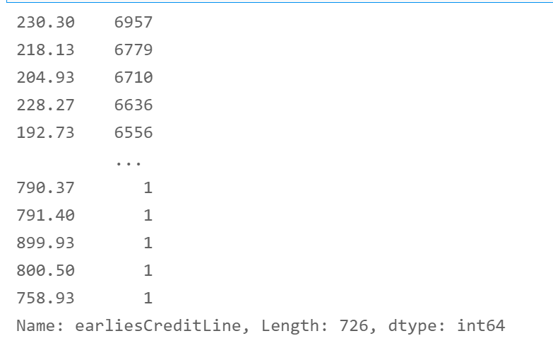
df['earliesCreditLine'] = df['earliesCreditLine'].apply(encoder1)
df['earliesCreditLine'].value_counts()
3. Save the file
train = df[df['train_test'] == 'train']
test = df[df['train_test'] == 'test']
del test['isDefault']
del train['train_test']
del test['train_test']
train.to_csv('train_process.csv')
test.to_csv('test_process.csv')
4. Data modeling
4.1.1 data viewing
# data processing
import numpy as np
import pandas as pd

# Data visualization
import matplotlib.pyplot as plt

# Feature selection and coding
from sklearn.preprocessing import LabelEncoder

# machine learning
from sklearn import model_selection, tree, preprocessing, metrics
from sklearn.ensemble import RandomForestClassifier, GradientBoostingClassifier
from sklearn.linear_model import LinearRegression, LogisticRegression, Ridge, Lasso, SGDClassifier
from sklearn.tree import DecisionTreeClassifier

# Grid search, random search
import scipy.stats as st
from sklearn.model_selection import GridSearchCV
from sklearn.model_selection import RandomizedSearchCV

# Model metrics (classification)
from sklearn.metrics import precision_recall_fscore_support, roc_curve, auc

# Warning handling
import warnings
warnings.filterwarnings('ignore')

# Draw on Jupyter
%matplotlib inline
train = pd.read_csv('train_process.csv')
test = pd.read_csv('test_process.csv')
train.shape, test.shape

train.columns,test.columns

# Delete Unnamed: 0
del train['Unnamed: 0']
del test['Unnamed: 0']
## In order to correctly evaluate the model performance, the data is divided into training set and test set, the model is trained on the training set, and the model performance is verified on the test set.
from sklearn.model_selection import train_test_split

## Select samples with categories 0 and 1 (excluding samples with category 2)
data_target_part = train['isDefault']
data_features_part = train[[x for x in train.columns if x != 'isDefault' and 'id']]

## The test set size is 20%, 80% / 20% points
x_train, x_test, y_train, y_test = train_test_split(data_features_part, data_target_part, test_size = 0.2, random_state = 2020)
x_train.head()
y_train.head()
4.1.1 selection algorithm
The following is the algorithm used
- Logistic Regression
- Random Forest
- Decision Tree
- Gradient Boosted Trees
# Draw AUC curve
import time
def plot_roc_curve(y_test, preds):
    fpr, tpr, threshold = metrics.roc_curve(y_test, preds)
    roc_auc = metrics.auc(fpr, tpr)
    plt.title('Receiver Operating Characteristic')
    plt.plot(fpr, tpr, 'b', label = 'AUC = %0.2f' % roc_auc)
    plt.legend(loc = 'lower right')
    plt.plot([0, 1], [0, 1],'r--')
    plt.xlim([-0.01, 1.01])
    plt.ylim([-0.01, 1.01])
    plt.ylabel('True Positive Rate')
    plt.xlabel('False Positive Rate')
    plt.show()
# Logistic Regression
clf1 = LogisticRegression(solver='sag', max_iter=100, multi_class='multinomial')
clf1.fit(x_train, y_train)
## The distribution on the training set and test set is predicted by the trained model
train_predict = clf1.predict(x_train)
test_predict = clf1.predict(x_test)
from sklearn import metrics

## The model effect is evaluated by accuracy [the proportion of the number of correctly predicted samples to the total number of predicted samples]
print('The accuracy of the Logistic Regression is:',metrics.accuracy_score(y_train,train_predict))
print('The accuracy of the Logistic Regression is:',metrics.accuracy_score(y_test,test_predict))

# Grid search
from sklearn.model_selection import GridSearchCV
param_grid = {
              'penalty': ['l2', 'l1'],
              'class_weight': [None, 'balanced'],
              'C': [0, 0.1, 0.5, 1],
                'intercept_scaling': [0.1, 0.5, 1]
             }

clf2 = LogisticRegression(solver='sag')
rfc = GridSearchCV(clf2, param_grid, scoring = 'neg_log_loss', cv=3, n_jobs=-1)
rfc.fit(x_train, y_train)
print(rfc.best_score_)
print(rfc.best_params_)

# Logistic Regression
clf1 = LogisticRegression(solver='sag', max_iter=100, penalty='l2',
class_weight=None, C=0.1, intercept_scaling=0.1)
model = clf1.fit(x_train, y_train)
## The distribution on the training set and test set is predicted by the trained model
train_predict = clf1.predict(x_train)
test_predict = clf1.predict(x_test)
from sklearn import metrics
## The model effect is evaluated by accuracy [the proportion of the number of correctly predicted samples to the total number of predicted samples]
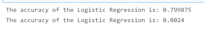
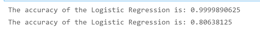
print('The accuracy of the Logistic Regression is:',metrics.accuracy_score(y_train,train_predict))
print('The accuracy of the Logistic Regression is:',metrics.accuracy_score(y_test,test_predict))
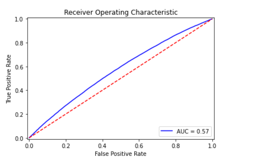
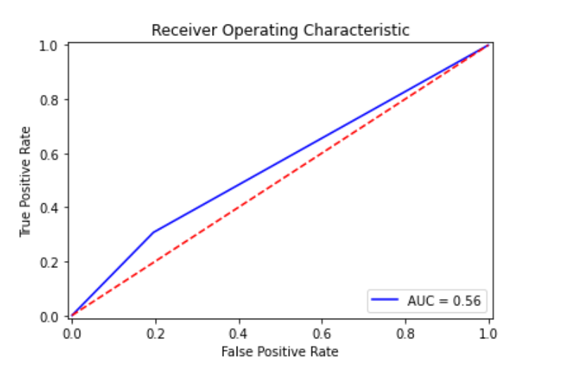
# Drawing
plot_roc_curve(y_test, model.predict_proba(x_test)[:,1])
# Random Forest

clf1 = RandomForestClassifier()
clf1.fit(x_train, y_train)
## The distribution on the training set and test set is predicted by the trained model
train_predict = clf1.predict(x_train)
test_predict = clf1.predict(x_test)
from sklearn import metrics

## The model effect is evaluated by accuracy [the proportion of the number of correctly predicted samples to the total number of predicted samples]
print('The accuracy of the Logistic Regression is:',metrics.accuracy_score(y_train,train_predict))
print('The accuracy of the Logistic Regression is:',metrics.accuracy_score(y_test,test_predict))
# Decision tree
clf1 = DecisionTreeClassifier()
model = clf1.fit(x_train, y_train)
## The distribution on the training set and test set is predicted by the trained model
train_predict = clf1.predict(x_train)
test_predict = clf1.predict(x_test)
from sklearn import metrics
## The model effect is evaluated by accuracy [the proportion of the number of correctly predicted samples to the total number of predicted samples]
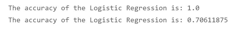
print('The accuracy of the Logistic Regression is:',metrics.accuracy_score(y_train,train_predict))
print('The accuracy of the Logistic Regression is:',metrics.accuracy_score(y_test,test_predict))
plot_roc_curve(y_test, model.predict_proba(x_test)[:,1])
# Gradient Boosting Trees

clf1 = GradientBoostingClassifier()
model = clf1.fit(x_train, y_train)
## The distribution on the training set and test set is predicted by the trained model
train_predict = clf1.predict(x_train)
test_predict = clf1.predict(x_test)
from sklearn import metrics

## The model effect is evaluated by accuracy [the proportion of the number of correctly predicted samples to the total number of predicted samples]
print('The accuracy of the Logistic Regression is:',metrics.accuracy_score(y_train,train_predict))
print('The accuracy of the Logistic Regression is:',metrics.accuracy_score(y_test,test_predict))

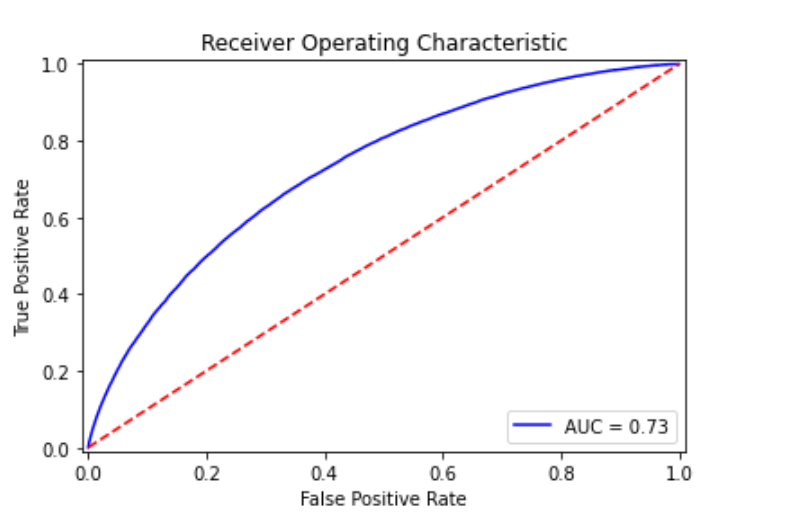
plot_roc_curve(y_test, model.predict_proba(x_test)[:,1])
End of code demonstration
3, Expand
If you are interested, you can also do feature fusion and model fusion, and do better feature engineering to make the AUC score of the model higher.