Point, knock on the blackboard

• First of all, this paper follows the traditional teaching, point to point! Only some functions or processing methods that are frequently used by individuals are introduced.
• The examples in this article are only used for demonstration. Generally, the examples do not modify the original data. If the code will modify the original data, it will be marked (modify on the original data). You must pay attention to whether you have modified the original data when using it yourself. Once an error is reported, first check whether your code has changed the original data.

# Original data not modified
df.drop('name', axis = 1)  
# Modify original data
df.drop('name', axis = 1, inplace=True)  
# Modify original data
df = df.drop('name', axis = 1)  

• pandas is powerful because it has a variety of data processing functions. Each function is combined with each other, flexible and changeable, and interacts with numpy, matplotlib, sklearn, > pyspark, sklearn and many other scientific computing libraries. It is the only way to really master the actual combat.
• It's not easy to be original, and the code word is also very tired. If you think the article is good, 💗 You must remember three times 💗 ~ Thank you in advance.

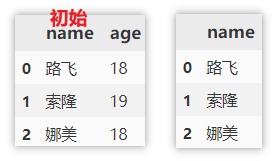
DataFrame creation

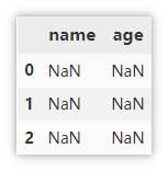
Create an empty DataFrame

Create an empty with three lines of empty data.

df = pd.DataFrame(columns=['name', 'age'], index=[0, 1, 2])

General DataFrame creation method

Only three common methods are introduced here: array creation, dictionary creation and external file creation. When reading common files, you can directly specify the file path. For xlsx files, there may be multiple sheets, so you need to specify sheets_ name .

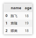
# Array creation
df = pd.DataFrame(data=[['Monkey D Luffy', 18],
                       ['Sauron', 19],
                       ['Nami', 18]],
                  columns=['name', 'age'])
# Create from dictionary
df = pd.DataFrame({'name': ['Monkey D Luffy','Sauron', 'Nami'],
					 'age':[18, 19, 18]})
# Create through external files, csv, xlsx, json, etc
df = pd.read_csv('XXX.csv')

DataFrame storage

Common storage methods (csv, json, excel, pickle)

Generally, you do not need to save the index when saving, because the index will be automatically generated when reading.

df.to_csv('test.csv', index=False)  # Ignore index
df.to_excel('test.xlsx', index=False)  # Ignore index
df.to_json('test.json')  # Save as json
df.to_pickle('test.pkl')  # Save in binary format

DataFrame view data information

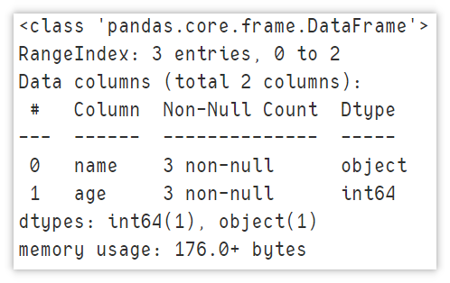
Display summary information

Before we use the DataFrame, we will view the data information. Personal preference info shows the row and column information of the dataset and the number of non null values in each column.

df.info()

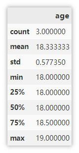
Display descriptive statistics

It can intuitively view the basic statistical information of the numerical column.

df.describe()

Show front / back n lines

5 rows are displayed by default. You can specify the number of rows to display.

df.head(n)  # You can specify an integer to output the first n lines
df.tail(n)  # You can specify an integer and output the following n lines

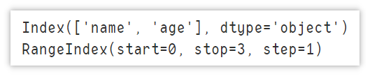
Display index and column information

Displays basic information about indexes and columns.

df.columns  # Column information
df.index  # Index information

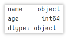
Displays the data type for each column

Displays the name of the column and the corresponding data type.

df.dtypes

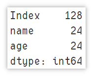
Displays the amount of memory used

Displays the amount of memory occupied by the column, in bytes.

df.memory_usage()

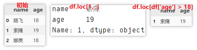
Locate a row of data

Important: both LOC and iloc use the method of specifying rows first and then columns, and the rows are separated from the list expression. For example: df.loc [:,:] get the data of all rows and all columns.

Locate using loc()

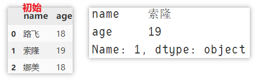
For example, to locate the data of [Solon], there are the following

df.loc[1, :]  # LOC [index, columns] row index, column name, return Series object
df.loc[df['age'] > 18]  # Return DataFrame object
# Or DF [DF ['age '] > 18]
# df.loc[df['name '] = =' Sauron ']

Positioning using iloc

Use iloc to get the data of the second row (the index starts from 0) and all columns.

df.iloc[1, :]  # iloc[index1, index2] row index, column index

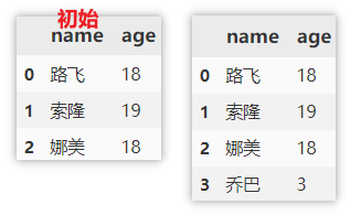
Add a row of data

Locate and add using loc

Use loc to locate the row with index = 3, and then assign a value (modify the original data)

df.loc[len(df)] = ['Joba', 3]

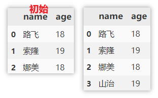
Add using append

append when adding data, you need to specify the column name and column value. If a column is not specified, NaN will be filled in by default.

df.append({'name': 'Yamaji', 'age': 19}, ignore_index=True)

Delete data

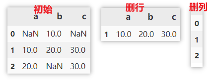
Delete columns based on column names

Use drop to delete a column, specify the axis to be deleted, and the name / index of the corresponding column / row.

df.drop('name', axis = 1)  # Delete single column
df.drop(['name', 'age'], axis = 1)  # Delete multiple columns

Delete rows based on index

The method of deleting columns is similar to that above, but the index is specified here.

df.drop(0, axis=0)  # Delete single line
df.drop([0, 1], axis=0)  # Delete multiple rows

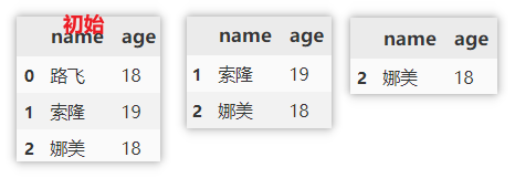
Locate and delete data using loc

First use loc to locate the data of a condition, then obtain the index index, and then use drop to delete it.

df.drop(df.loc[df['name'] == 'Nami'].index, axis=0)  # Delete the anchored row

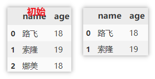
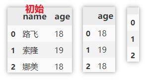
Delete columns using del

del is used to modify the original data, which should be paid attention to.

del df['age']

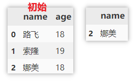
Delete rows and columns at the same time

drop can also specify rows and columns to delete at the same time. Here, delete the first and second rows and delete the age column.

df.drop(columns=['age'], index=[0, 1])

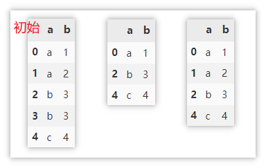
Delete duplicate values

• When a subset is specified, the duplicate is removed according to the specified column as a reference. That is, if the a values of two rows are the same, the row that appears the second time will be deleted and only the first row will be retained
• If you do not specify a subset, all columns will be used as references for de duplication. Only two rows of data are identical will be de duplicated.

df.drop_duplicates(subset=['a'], keep='first')
df.drop_duplicates(keep='first')

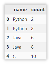
Screening duplicate values

Sample data

df = pd.DataFrame({'name':['Python',
                        'Python',
                        'Java',
                        'Java',
                        'C'],
                   'count': [2, 2, 6, 8, 10]})

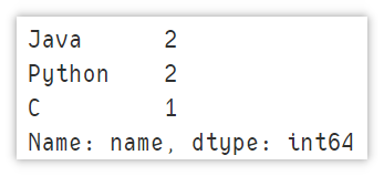
Determine whether a column has duplicate values

Use values_counts() counts the occurrence times of each value in the column. The results are arranged in descending order by default. You only need to judge whether the occurrence times of the values in the first row is 1 to judge whether there are duplicate values.

df['a'].value_counts()

Using drop_duplicates() deletes duplicate values and only keeps the first value. It determines whether the processed value is equal to the original df. If False, it indicates that there are duplicate values.

df.equals(df.drop_duplicates(subset=['a'], keep='first'))

False

Judge whether there are duplicate rows in the DataFrame

Drop is also used_ Duplicates() deletes duplicate values and only keeps the values that appear for the first time. At this time, the subset parameter is not used to set the columns. The default is all columns. Judge whether the processed values are equal to the original df. If False, it indicates that there are duplicate values.

df.equals(df.drop_duplicates(keep='first'))

False

Count the number of duplicate lines

Note that the statistics here refer to all columns. Only two rows are identical will be judged as duplicate rows, so the statistical result is 1.

len(df) - len(df.drop_duplicates(keep="first"))

1

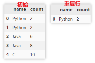
Show duplicate data rows

Delete the duplicate rows first, keep only the first row, get a unique dataset of rows, and then use drop_duplicates() deletes all duplicate data in df, and does not retain the duplicate value for the first time. Merge the above two result sets and use drop_duplicates() de duplicates the newly generated data set to obtain the data of duplicate rows.

df.drop_duplicates(keep="first")\
  .append(df.drop_duplicates(keep=False))\
  .drop_duplicates(keep=False)

Missing value processing

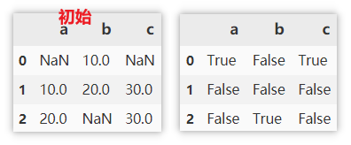
Find missing values

The missing value is True and the non missing value is False.

df.isnull()

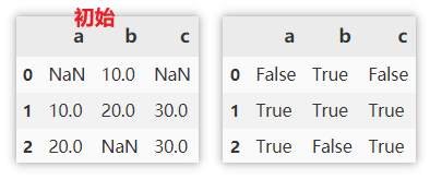
Find non missing values

The non missing value is True and the missing value is False.

df.notnull()

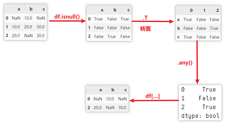
Show rows with missing values

. isnull: find the missing value, mainly to mark the position of the missing value as True.
. T: transpose rows and columns to prepare for the next step any.
. any: returns True if one True is satisfied in a sequence.

df[df.isnull().T.any()]

Delete missing values

There are a lot of parameters to pay attention to here, which will be emphasized here.

• axis: 0 rows, 1 columns
• how:
  • any: if NaN exists, delete the row or column.
  • All: if all values are NaN, delete the row or column.
• thresh: Specifies the number of NaN. It is deleted only when the number of NaN reaches.
• Subset: the data range to be considered. For example, when deleting missing rows, use subset to specify the referenced columns. All columns are selected by default.
• inplace: whether to modify the original data.

# Delete a row if it has missing values
df.dropna(axis=0, how='any')  
# Delete a column if it has missing values
df.dropna(axis=1, how='any')  

Fill in missing values

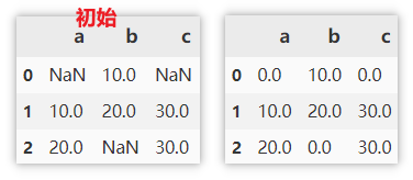
Numeric or string padding

Directly specify the number or string to populate.

df.fillna(0)

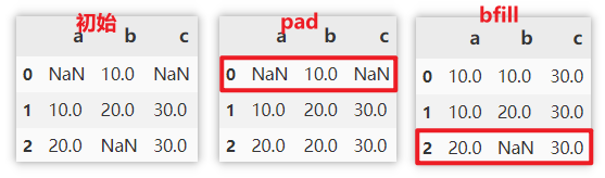
Fill with values before / after missing values

• It is filled with the previous value of the missing value (the value above the column). If the missing value is in the first row, it is not filled
• It is filled with the last value of the missing value (the value below the column). If the missing value is in the last row, it is not filled

df.fillna(method='pad')
df.fillna(method='bfill')

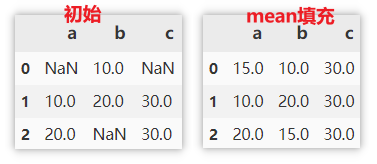
Fill with the mean / median of the column in which the missing value is located

It can be populated with the statistics of this column. Such as filling with mean, median, max, min, sum, etc.

df.fillna(df.mean())

Column operation

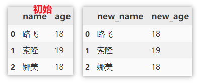
Modify column name

df.columns directly specifies a new column name to replace all column names. (modify the original data)
rename() needs to specify the original name and new name to replace.

df.columns = ['new_name', 'new_age']
df.rename(columns=({'name':'new_name','age':'new_age'}))

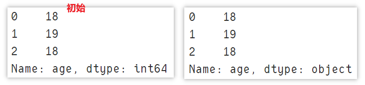
Modify column type

Use astype to modify the column type.

df['age'].astype(str)

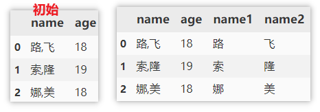
Split columns to get multiple columns

Split can only split character string columns.

df[['name1', 'name2']] = df['name'].str.split(',', expand=True)

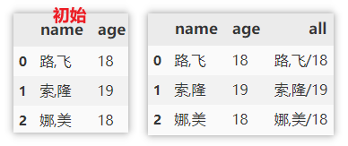
Merge multiple columns into a new column

Similarly, only columns of string type can be merged.

df['all'] = df['name'] + '/' + df['age'].astype(str)

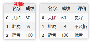
Partition numeric columns

For the value column, it may be necessary to change these values into label values according to the specified range, such as passing and failing indicators of the product, excellent performance, etc. To use, you need to specify the value column, the critical value of each label, the opening and closing of the critical value (in the example: the default is left=True, specify right=False, that is, close left and open right), and finally specify the name of the label.

df['evaluate'] = pd.cut(df['achievement'], [0, 60, 80, np.inf],
			 right=False, labels=['fail,', 'good', 'excellent'])

sort

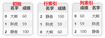
index order

Sort row index in descending order

df.sort_index(axis=0, ascending=False)

Sort column index in descending order

df.sort_index(axis=1, ascending=False)

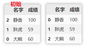
Reset index

Reorder the index so that the original index is not retained.

df.reset_index(drop=True)

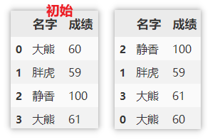
Value sorting

First sort by name in descending order, and then sort the scores under the same name in descending order.

df.sort_values(by=['name', 'achievement'], axis=0, ascending=False)

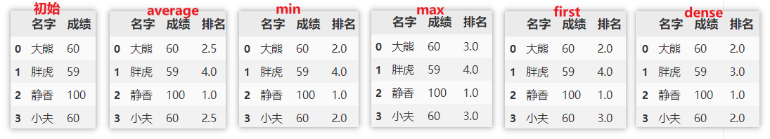
Create ranking column

rank is used for ranking. The value meaning of the main parameter method is as follows:

method	meaning
average	By default, in the group with the same ranking, the average ranking (average) is assigned to each value, and there is a jump between the rankings
min	Using the smallest ranking in the group, there is a jump between the rankings
max	Using the largest ranking in the group, there is a jump between the rankings
first	The values are ranked according to the order in which they appear in the original data, and there is a jump between the rankings
dense	The ranking of the same group is the same, and there is no jump between the rankings

Now rank each row of data according to the score column and create a new ranking column. Several ranking methods are given below.

df['ranking'] = df['achievement'].rank(method='average', ascending=False)

grouping

Grouping statistics of rows

Now calculate the scores in groups, and calculate the sum, mean and maximum respectively.

df.groupby(['name']).sum()
df.groupby(['name']).mean()
df.groupby(['name']).max()

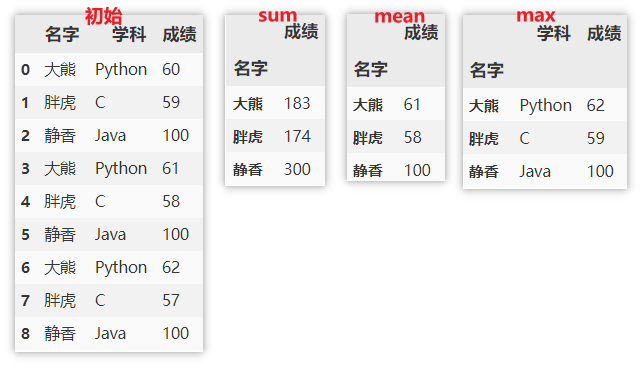
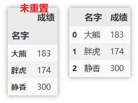
Note: the index is the name at this time. If you want to reset the index, you can use the following method.

df.groupby(['name']).sum().reset_index()

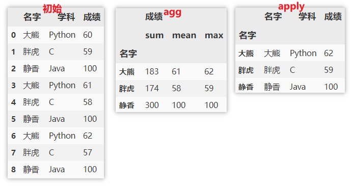
Use different statistical functions for different columns

agg() specifies that the function is used on a sequence of numbers and then returns a scalar value.
apply() is the process of splitting the data > > > then applying > > > and finally summarizing (only a single function can be applied). Returns multidimensional data.

df.groupby(['name']).agg({'achievement':['sum','mean','max']})
df.groupby(['name']).apply(max)

DataFrame merge

The merge functions in pandas are mainly: merge(), concat(), append(), which are generally used to connect two or more dataframes. Concat (), append () is used to connect DataFrame objects vertically and merge () is used to connect DataFrame objects horizontally.

Comparison of the three:

concat()

• Connecting multiple dataframes
• Set a specific key

append()

• Connecting multiple dataframes

merge()

• Specify columns to connect to the DataFrame

merge()

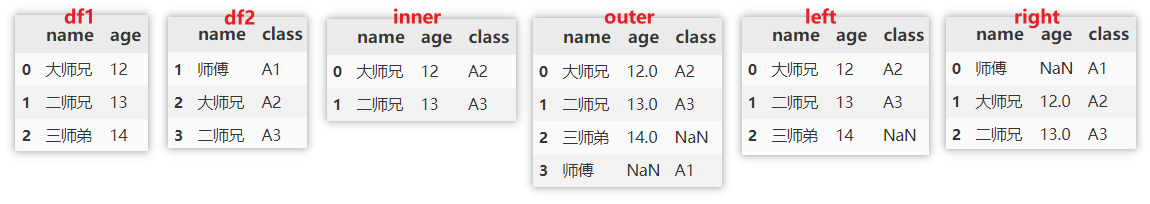
If on is specified, the column must appear in the two dataframes at the same time. The default value is the intersection of the two DataFrame columns. In this example, even if on is not specified, the actual default value will be merged according to the name column.
how parameter details:

• inner: take the intersection according to the column specified by on.
• outer: takes the union set according to the column specified by on.
• Left: merge according to the column specified by on and left join.
• Right: merge according to the column specified by on and right join.

pd.merge(df1, df2, on='name', how = "inner")
pd.merge(df1, df2, on='name', how = "outer")
pd.merge(df1, df2, on='name', how = "left")
pd.merge(df1, df2, on='name', how = "right")

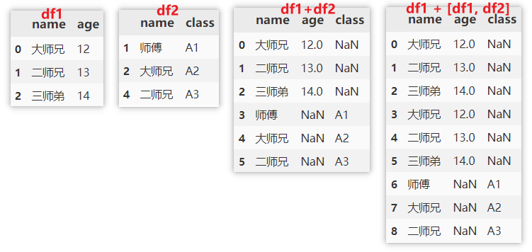
concat()

concat() can merge multiple dataframes. You can choose vertical merge or horizontal merge according to the actual situation. See the following example for details.

# Vertical merging and intersection of multiple dataframes
pd.concat([df1, df2], ignore_index=True, join='inner',axis=0)
# Vertical merge and union of multiple dataframes
pd.concat([df1, df2], ignore_index=True, join='outer',axis=0)
# Horizontal merging and intersection of multiple dataframes
pd.concat([df1, df2], ignore_index=False, join='inner',axis=1)
# Horizontal merge and union of multiple dataframes
pd.concat([df1, df2], ignore_index=False, join='outer',axis=1)

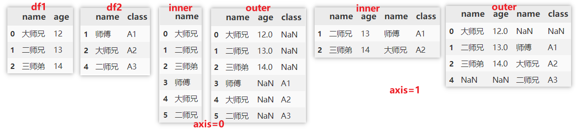
In addition, you can also specify a key to add the name of the original data at the index position.

pd.concat([df1, df2], ignore_index=False, join='outer', keys=['df1', 'df2'])

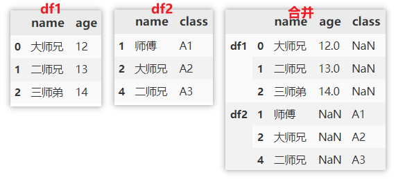
append()

append() is often used for vertical merging, or merging multiple dataframes.

df1.append(df2, ignore_index=True)
df1.append([df1, df2], ignore_index=True)

DataFrame time processing

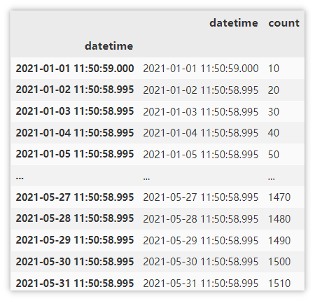
Sample data

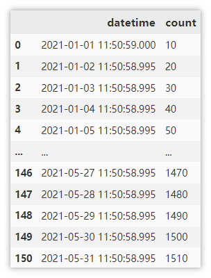
Convert character string into time series

Sometimes the time read from csv or xlsx files is of the type of string (Object). In this case, it needs to be converted into the type of datetime to facilitate subsequent time processing.

pd.to_datetime(df['datetime'])

Index time column

For most time series data, we can use this column as an index to maximize the use of time. Here drop=False, choose not to delete the datetime column.

df.set_index('datetime', drop=False)

Get the data of January through the index, and the first five lines are displayed here.

df.loc['2021-1'].head()

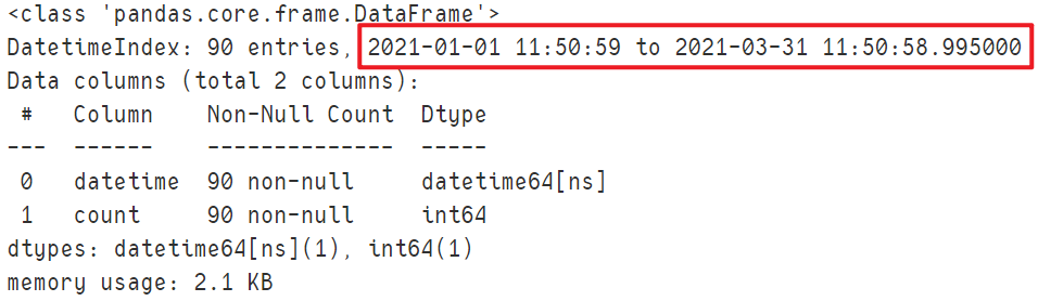
Obtain the data from January to march through the index.

df.loc['2021-1':'2021-3'].info()

Get each attribute of time

Here are the attributes that may be used in general requirements, as well as examples of various methods.

Common properties	describe
date	get date
time	Get time
year	Get year
month	Get month
day	Get days
hour	Get hours
minute	Get minutes
second	Get seconds
dayofyear	What day of the year is the data in
weekofyear	What week of the year is the data in (the new version uses isocalendar().week)
weekday	The day of the week on which the data is in (the number Monday is 0)
day_name()	What day of the week is the data in
quarter	What quarter of the year is the data in
is_leap_year	Is it a leap year

Here, select the date in line 100 as an example, and the results of each attribute are displayed in the form of comments.

df['datetime'].dt.date[100]
# datetime.date(2021, 4, 11)
df['datetime'].dt.time[100]
# datetime.time(11, 50, 58, 995000)
df['datetime'].dt.year[100]
# 2021
df['datetime'].dt.month[100]
# 4
df['datetime'].dt.day[100]
# 11
df['datetime'].dt.hour[100]
# 11
df['datetime'].dt.minute[100]
# 50
df['datetime'].dt.second[100]
# 58
df['datetime'].dt.dayofyear[100]
# 101
df['datetime'].dt.isocalendar().week[100]
# 14
df['datetime'].dt.weekday[100]
# 6
df['datetime'].dt.day_name()[100]
# 'Sunday'
df['datetime'].dt.quarter[100]
# 2
df['datetime'].dt.is_leap_year[100]
# False

resample()

Resampling is divided into down sampling and up sampling.

Downsampling means that the time frequency of sampling is lower than that of the original time series. At the same time, it is an aggregation operation. Looking at the example, let's get the average value of the count column for each quarter. Q stands for quarter, which means sampling by quarter.

df.resample('Q',on='datetime')["count"].mean()

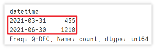
Note: the maximum output time at this time is 06-30, not 05-31 in the actual data. However, it does not affect the calculation.

Upsampling is opposite to downsampling. It means that the time frequency of sampling is higher than that of the original time series, which is equivalent to obtaining time data in finer latitudes. However, this often leads to a large number of null values in the data, which are not used in practice. I won't explain it here.

DataFrame traversal mode

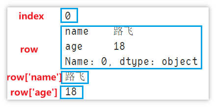
iterrows() - traverse rows (index, column value sequence)

Traverse by row to obtain the row index and column value sequence. The speed is slow. Look at the example directly.

for index, row in df.iterrows():
    print(index)
    print(row)
    print(row['name'])
    print(row['age'])
    break # Used in the demonstration, only one line is displayed

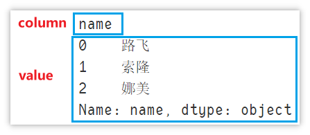
iteritems() - traversal (column name, value)

Traverse by column to obtain the column name and the value of the column.

for column, value in df.iteritems():
    print(column)
    print(value)
    break # Used in the demonstration, only one line is displayed

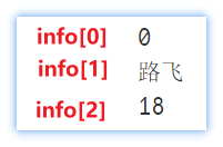
itertuples() - traverse rows (index, column value A, column value B...)

Traverse by row to obtain the index and column value of the row. The difference from iterrows is that the index and column value are included together, and info[0] is used to obtain the index

for info in df.itertuples():
    print(info[0])
    print(info[1])
    print(info[2])
    break # Used in the demonstration, only one line is displayed

This is all the content of this article, if it feels good. ❤ Remember to support the third company!!! ❤


In the future, we will continue to share all kinds of dry goods. If you are interested, you can pay attention and don't get lost ~.

People like me who love fans will of course give 100 million little benefits to my fans. Pay attention to the small cards below and get the blogger's various article source code and data analysis dry goods!

👇 👇 👇