Author home page( Silicon based workshop of slow fire rock sugar): Slow fire rock sugar (Wang Wenbing) blog silicon based workshop of slow fire rock sugar _csdnblog
Website of this article: https://blog.csdn.net/HiWangWenBing/article/details/120600611
catalogue
Introduction deep learning model framework
Chapter 1 business area analysis
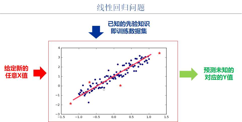
one point one Step 1-1: business domain analysis
1.2 steps 1-2: Business Modeling
1.3 code instance preconditions
Chapter 2 definition of forward operation model
two point one Step 2-1: dataset selection
two point two Step 2-2: Data Preprocessing
2.3 step 2-3: neural network modeling
2.4 steps 2-4: neural network output
Chapter 3 definition of backward operation model
3.1 step 3-1: define the loss function
three point two Step 3-2: define the optimizer
3.4 step 3-4: model validation
3.5 step 3-5: Model Visualization
4.1 step 4-1: model deployment
Introduction deep learning model framework
 https://blog.csdn.net/HiWangWenBing/article/details/120462734
Chapter 1 business area analysis
one point one Step 1-1: business domain analysis
1.2 steps 1-2: Business Modeling
1.3 code instance preconditions
#Environmental preparation
import numpy as np              # numpy array library
import math                     # Mathematical operation Library
import matplotlib.pyplot as plt # Drawing library

import torch             # torch base library
import torch.nn as nn    #  torch neural network library

print("Hello World")
print(torch.__version__)
print(torch.cuda.is_available())
Hello World 1.8.0 False
Chapter 2 definition of forward operation model
two point one Step 2-1: dataset selection
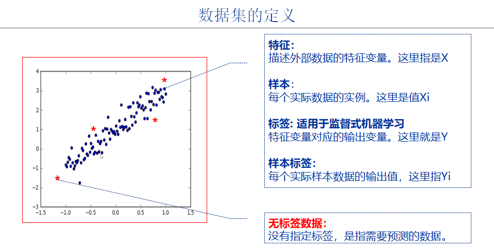
There is no need to use the existing open source data set, just build the data set yourself.
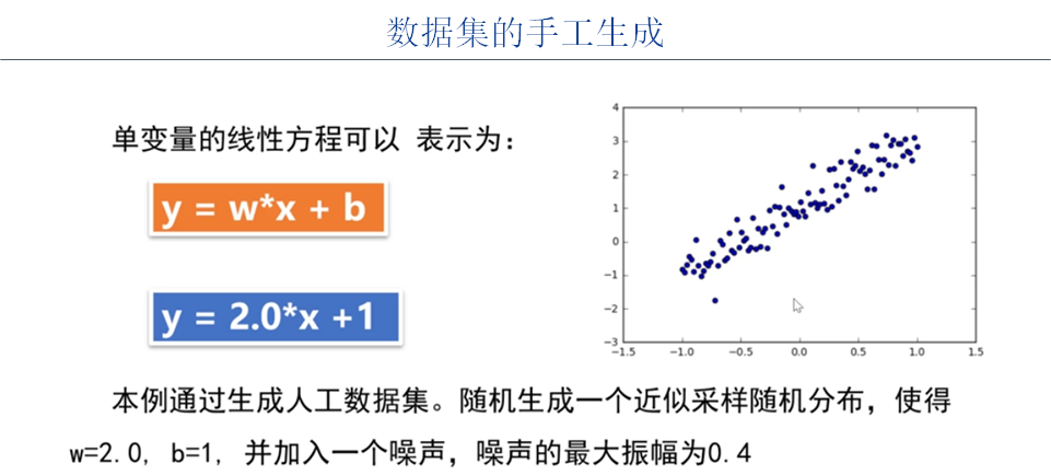
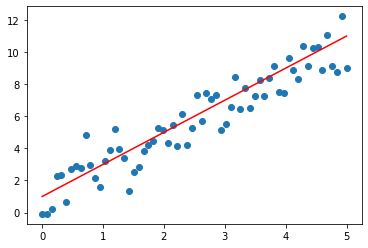
#2-1 preparing data sets
x_sample = np.linspace(0, 5, 64)

noise = np.random.randn(64)
y_sample = 2 * x_sample + 1 + noise

y_line = 2 * x_sample + 1

#Visual data
plt.scatter(x_sample, y_sample)
plt.plot(x_sample, y_line,'red')
two point two Step 2-2: Data Preprocessing
(1) Convert numpy one-dimensional data into two-dimensional sample data
(2) Convert numpy sample data into torch sample data
# 2-2 data preprocessing
print("Numpy Shape of original sample")
print(x_sample.shape)
print(y_sample.shape)
# Convert one-dimensional linear data into two-dimensional sample data, and each sample data is one-dimensional
print("\nNumpy Shape of training sample")
x_numpy = x_sample.reshape(-1, 1).astype('float32')
y_numpy = y_sample.reshape(-1, 1).astype('float32')
print(x_numpy.shape)
print(y_numpy.shape)
# Convert numpy sample data to pytorch sample data
print("\ntorch Shape of training sample")
x_train = torch.from_numpy(x_numpy)
y_train = torch.from_numpy(y_numpy)
print(x_train.shape)
print(y_train.shape)
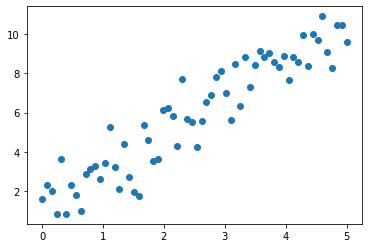
plt.scatter(x_train, y_train)Shape of Numpy original sample (64,) (64,) Shape of Numpy training sample (64, 1) (64, 1) Shape of torch training sample torch.Size([64, 1]) torch.Size([64, 1])
Out[3]:
<matplotlib.collections.PathCollection at 0x1fdc56524f0>
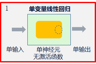
2.3 step 2-3: neural network modeling
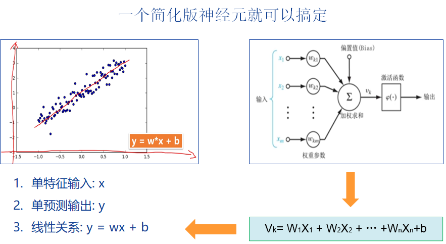
The neural network model here is a linear neuron with single input (size=1), single output (size=1) and no activation function.
# 2-3 define network model
print("Define and initialize the model")
w = Variable(torch.randn(1), requires_grad=True)
b = Variable(torch.randn(1), requires_grad=True)
print(w, w.data)
print(b, b.data)

def linear_mode(x):
    return (w * x + b)

model = linear_mode
Define and initialize the model tensor([0.1358], requires_grad=True) tensor([0.1358]) tensor([0.4257], requires_grad=True) tensor([0.4257])
2.4 steps 2-4: neural network output
# 2-4 define network prediction output
y_pred = linear_mode(x_train)
print(y_pred.shape)
torch.Size([64, 1])
Note: the output is one-dimensional data of 64 samples
Chapter 3 definition of backward operation model
3.1 step 3-1: define the loss function
The MSE loss function used here
# 3-1 define the loss function:
# loss_fn= MSE loss
def MSELoss(y_, y):
    return (torch.mean((y_ - y)**2))

loss_fn = MSELoss

print(loss_fn)
<function MSELoss at 0x00000197671FD0D0>
three point two Step 3-2: define the optimizer
# 3-2 defining the optimizer
Learning_rate = 0.01     #Learning rate

# lr: indicates the learning rate
def optimizer_SGD_step(lr):
    w.data = w.data - lr * w.grad.data
    b.data = b.data - lr * b.grad.data

optimizer = optimizer_SGD_step

print(optimizer)
<function optimizer_SGD_step at 0x00000197671FD430>
3.3 step 3-3: model training
# 3-3 model training
w = Variable(torch.randn(1), requires_grad=True)
b = Variable(torch.randn(1), requires_grad=True)

# Define the number of iterations
epochs = 500

loss_history = [] #loss data during training
w_history = []    #Values of w parameters during training
b_history = []    #b parameter value during training

for i in range(0, epochs):

    #(1) Forward calculation
    y_pred = model(x_train)

    #(2) Calculate loss
    loss = loss_fn(y_pred, y_train)

    #(3) Reverse derivation
    loss.backward(retain_graph=True)

    #(4) Reverse iteration
    optimizer_SGD_step(Learning_rate)

    #(5) Reset the gradient of the optimizer
    #optimizer.zero_grad()
    w.grad.zero_()
    b.grad.zero_()

    #Record iteration data
    loss_history.append(loss.data)
    w_history.append(w.data)
    b_history.append(b.data)

    if(i % 100 == 0):
        print('epoch {}  loss {:.4f}'.format(i, loss.item()))

print("\n Iteration completion")
print("\n After training w Parameter value:", w)
print("\n After training b Parameter value:", b)
print("\n Minimum loss value:", loss)
print(len(loss_history))
print(len(w_history))
print(len(b_history))
epoch 0 loss 42.0689 epoch 100 loss 1.0441 epoch 200 loss 1.0440 epoch 300 loss 1.0439 epoch 400 loss 1.0439 Iteration completion After training w parameter value: Parameter containing: tensor([[1.8530]], requires_grad=True) 1.8529784679412842 After training, b parameter value: Parameter containing: tensor([1.2702], requires_grad=True) 1.2701895236968994 Minimum loss value: tensor (1.0439, grad_fn = < mselossbackward >) 1.0438624620437622 500 500 500
3.4 step 3-4: model validation
NA
3.5 step 3-5: Model Visualization
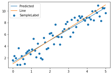
# 3-4 visual model data
#The model returns the total tensors, including grad_fn. The tensors extracted from data are pure tensors
y_pred = model(x_train).data.numpy().squeeze()
print(x_train.shape)
print(y_pred.shape)
print(y_line.shape)

plt.scatter(x_train, y_train, label='SampleLabel')
plt.plot(x_train, y_pred, label='Predicted')
plt.plot(x_train, y_line, label='Line')

plt.legend()
plt.show()
torch.Size([64, 1])
(64,)
(64,)
#Display historical data of loss
plt.plot(loss_history, "r+")
plt.title("loss value")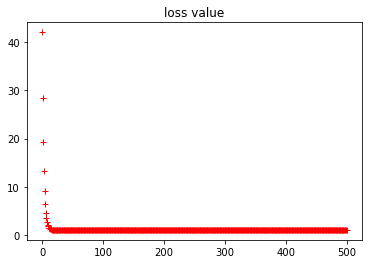
#Displays historical data for w parameters
plt.plot(w_history, "r+")
plt.title("w value")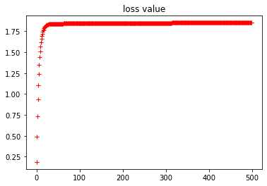
#Displays the historical data of the b parameter
plt.plot(b_history, "r+")
plt.title("b value")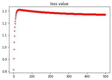
Chapter 4 model deployment
4.1 step 4-1: model deployment
NA
Author home page( Silicon based workshop of slow fire rock sugar): Slow fire rock sugar (Wang Wenbing) blog silicon based workshop of slow fire rock sugar _csdnblog
Website of this article: https://blog.csdn.net/HiWangWenBing/article/details/120600611