Multisensor fusion localization Chapter 8 advanced fusion method based on filtering
Reference blog: Deep Blue College - multi-sensor fusion positioning - Chapter 7 operation
 1. Environment configuration
1.1 protoc ol version problem
The protoc version used in the previous chapters is 3.14, and the proto version used in Chapter 7 is 3.15
Solution: you need to install a new version of proto 3.15x according to Chapter IV methods Generate the corresponding file.
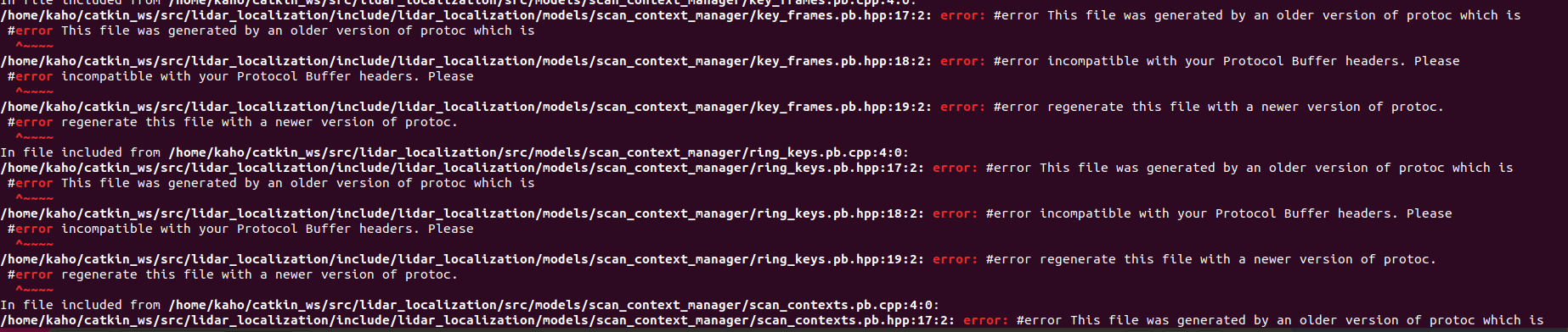
Regenerate proto based on its own base environment protobuf according to the method in GeYao README:
Open lidar_localization/config/scan_context folder, enter the following command to generate pb file
protoc --cpp_out=./ key_frames.proto
protoc --cpp_out=./ ring_keys.proto
protoc --cpp_out=./ scan_contexts.proto
mv key_frames.pb.cc key_frames.pb.cpp
mv ring_keys.pb.cc ring_keys.pb.cpp
mv scan_contexts.pb.cc scan_contexts.pb.cpp
Modify the generated three. Pb.cpp files respectively. As follows, ring_keys.pb.cpp as an example.
// Generated by the protocol buffer compiler.  DO NOT EDIT!
// source: ring_keys.proto

#define INTERNAL_SUPPRESS_PROTOBUF_FIELD_DEPRECATION
#include "ring_keys.pb.h" Replace with  #include "lidar_localization/models/scan_context_manager/ring_keys.pb.h"

#include <algorithm>
Then, replace lidar with the. pb.h file generated in the above steps_ localization/include/lidar_ localization/models/scan_ context_ manager
A file with the same name in.
Replace the. pb.cpp file (Note: it needs to be cut to ensure that the newly generated files in the config file are transferred to the corresponding directory and cannot appear repeatedly) lidar_ localization/src/models/scan_ context_ A file with the same name in manager.
1.2 lack of fmt Library
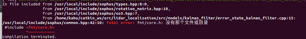
git clone https://github.com/fmtlib/fmt
cd fmt/
mkdir build
cd build
cmake ..
make
sudo make install
Error occurred during compilation_ state_ kalman_ Filter. CPP: (. Text. Unlikely + 0x84): for 'FMT:: V8:: detail:: assert'_ Failure (char const, int, char const) 'undefined reference**
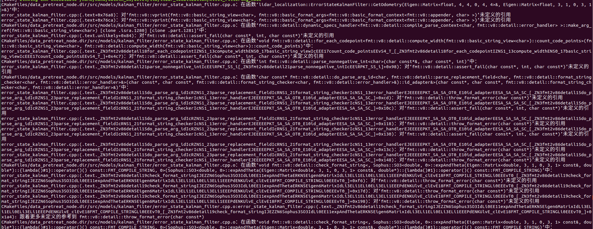
Reference website: undefined reference to `vtable for fmt::v7::format_error'
cd catkin_ws/src/lidar_localization/cmake/sophus.cmake
Add fmt to list append
#  sophus.cmake
find_package (Sophus REQUIRED)

include_directories(${Sophus_INCLUDE_DIRS})
list(APPEND ALL_TARGET_LIBRARIES ${Sophus_LIBRARIES} fmt)
1.3 glog lacks the dependency of gflag
logging.cc:(.text+0x6961): undefined reference to 'Google:: flagregister:: flagregister (char const *, char const *, char const *, bool *, bool *')
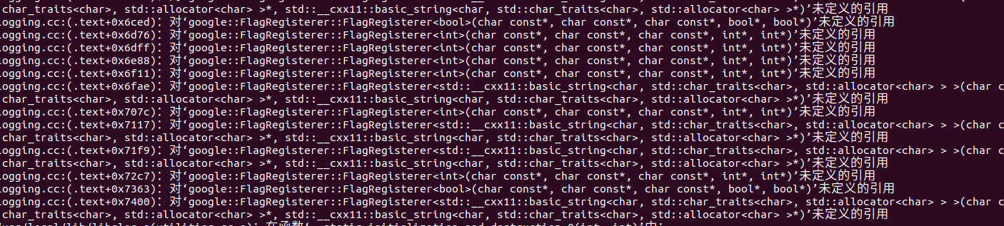
#Solution: open glog.cmake and change the end to
list(APPEND ALL_TARGET_LIBRARIES ${GLOG_LIBRARIES} libgflags.a libglog.a)
2. Add the error state Kalman filter of the transport model
FILE: lidar_localization/src/model/kalman_filter/error_state_kalman_filter.cpp
2.1 fusion encoder model
The encoder can provide an additional wheel speed odometer. In the case of not very high frequency encoder, it can be used as a constraint edge to carry out kalman fusion by providing linear speed (system b) into the observation equation in the previous chapter.
be careful:
1. The linear speed provided by the encoder is relatively accurate, but the angular speed is not very accurate(There is slip when turning),Angular velocity should not be used as observation edge.
2.Encoder participation fusion,There is another way of integration,That is, the encoder is not used for observation,But with IMU State prediction together,Then with
 The observations provided by other sensors are filtered and fused. The specific idea is IMU Provide angular velocity,The encoder provides linear speed,It is assumed that the frequency is the same and the timestamp is aligned,And the external parameters have been calibrated,Then they can be directly regarded as a new sensor that can obtain attitude and position through solution.
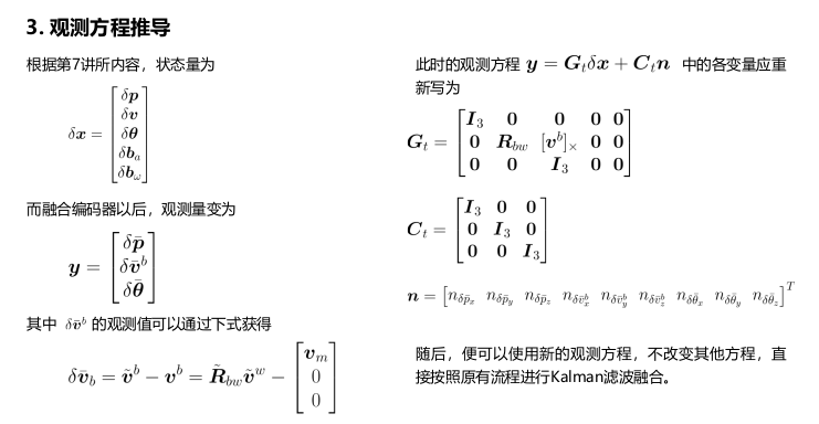
2.2 add motion constraint model (pseudo observation)
In the vehicle coordinate system (front upper left), on the basis of no encoder hardware, the motion attributes of the four-wheel chassis can be used for constraints. Under normal circumstances, the vehicle only has forward (x) speed, and the observations in y and z directions are 0. Therefore, two constraint edges Vy and Vz can be added to the observation.
2.3 coding
FILE: catkin_ws/src/lidar_localization/src/models/kalman_filter/error_state_kalman_filter.cpp
2.3.1 calling correcterrorextimation
  case MeasurementType::POSE_VEL:
    CorrectErrorEstimationPoseVel(
        measurement.T_nb,
        measurement.v_b, measurement.w_b,
         Y, G, K
    );
    break;
2.3.2 correcterrorextimationposvel calculation Y, G, K
be careful:
-
V entered in the correcterrorextimationposvel function_ B is from inertial navigation. Because KITTI data set has no wheel speed odometer information, if the measurement velocity input is v when making the fusion motion constraint model_ B. It can be considered that the observation is taken from ins.
-
Use the motion constraint of the vehicle (vy = 0;vz = 0) as the pseudo observation constraint, as shown below:
// Eigen:: Vector3D v_b_ = {v_b [0], 0, 0}; / / measurement velocity (body system), pseudo observation (vy, VZ = 0)
Eigen::Vector3d  v_b_  =  v_b;           //  Measurement velocity (body system), integration velocity (vx from INS)
void ErrorStateKalmanFilter::CorrectErrorEstimationPoseVel(          //  Calculate Y, G, K
    const Eigen::Matrix4d &T_nb, const Eigen::Vector3d &v_b, const Eigen::Vector3d &w_b,
    Eigen::VectorXd &Y, Eigen::MatrixXd &G, Eigen::MatrixXd &K
) {
    //
    // TODO: set measurement: calculate the observed delta pos and delta ori
    //
    // Eigen:: Vector3D v_b_ = {v_b [0], 0, 0}; / / measurement velocity (body system), pseudo observation (vy, VZ = 0)
    Eigen::Vector3d  v_b_  =  v_b;           //  Measurement velocity (body system), integration velocity (vx from INS)

    Eigen::Vector3d  dp  =  pose_.block<3,  1>(0,  3)  -   T_nb.block<3,  1>(0,  3);
    Eigen::Matrix3d  dR  =  T_nb.block<3,  3>(0, 0).transpose() *  pose_.block<3, 3>(0, 0) ;
    Eigen::Vector3d  dv  =   T_nb.block<3,  3>(0, 0).transpose() *vel_  -  v_b_ ;                  //  delta v strictly speaking, the observation here is vx given by inertial navigation
    // TODO: set measurement equation:
    Eigen::Vector3d  dtheta  =  Sophus::SO3d::vee(dR  -  Eigen::Matrix3d::Identity() );
    YPoseVel_.block<3, 1>(0, 0)  =  dp;          //    delta  position
    YPoseVel_.block<3, 1>(3, 0)  =  dv;           //   delta   velocity  s
    YPoseVel_.block<3, 1>(6, 0)  =  dtheta;          //   Misalignment angle
    Y = YPoseVel_;
    //   set measurement  G
    GPoseVel_.setZero();
    GPoseVel_.block<3, 3>(0, kIndexErrorPos)  =  Eigen::Matrix3d::Identity();
    GPoseVel_.block<3, 3>(3, kIndexErrorVel)   =   T_nb.block<3,  3>(0, 0).transpose();
    GPoseVel_.block<3, 3>(3, kIndexErrorOri)   =   Sophus::SO3d::hat( T_nb.block<3,  3>(0, 0).transpose() *vel_  ) ;
    GPoseVel_.block<3 ,3>(6, kIndexErrorOri)   =  Eigen::Matrix3d::Identity();
    G  =   GPoseVel_;
    //   set measurement  C
    CPoseVel_.setIdentity();
    Eigen::MatrixXd  C  =   CPoseVel_;
    // TODO: set Kalman gain:
    Eigen::MatrixXd R = RPoseVel_;    //  Observation noise
    K =  P_  *  G.transpose() * ( G  *  P_  *  G.transpose( )  +  C * RPoseVel_*  C.transpose() ).inverse() ;
}
2.3.2 write the updated vel_b to txt for comparison
/*********************write  data  to  txt********************/
#include <list>
#include <sstream>
#include <fstream>
#include <iomanip>
#define    DEBUG_PRINT

std::ofstream  fused;
std::ofstream  fused_vel;
std::ofstream  fused_cons;

bool CreateFile(std::ofstream& ofs, std::string file_path) {
    ofs.open(file_path, std::ios::out);                          //  Use std::ios::out to achieve coverage
    if(!ofs)
    {
        std::cout << "open csv file error " << std::endl;
        return  false;
    }
    return true;
}
/* write2txt  */
void WriteText(std::ofstream& ofs, Eigen::Vector3d data){
    ofs << std::fixed  <<  data[0] << "\t" <<  data[1]  << "\t "  <<  data[2] <<  "\t"  <<  std::endl;
}
call
  /*init  debug print file */
  #ifdef    DEBUG_PRINT
      char fused_path[] = "/home/kaho/shenlan_ws/src/lidar_localization/slam_data/trajectory/fused.txt";
      char fused_vel_path[] = "/home/kaho/shenlan_ws/src/lidar_localization/slam_data/trajectory/fused_vel.txt";
      char fused_cons_path[] = "/home/kaho/shenlan_ws/src/lidar_localization/slam_data/trajectory/fused_cons.txt";
      CreateFile(fused, fused_path );
  #endif
  ------------------------------------------------------------------------------------
      /*print  vel(body)*/
  #ifdef  DEBUG_PRINT
      Eigen::Vector3d  vel_print_ =   pose_.block<3, 3>(0, 0).transpose() *  vel_;       //  convert  kalman  filter velocity  to  body axis
      WriteText(fused, vel_print_ );   // Write into folder
  #endif
2.4 EVO evaluation and v_b comparison after update
evo evaluation instruction
# set up session:
source devel/setup.bash
# save odometry:
rosservice call /save_odometry "{}"
# run evo evaluation:
# a. fused does not input the motion model, outputs the evaluation results, and stores them in zip format:
evo_ape kitti ground_truth.txt fused.txt -r full --plot --plot_mode xy  --save_results ./fused.zip
# b. fused_vel velocity observation outputs the evaluation results and stores them in zip format:
evo_ape kitti ground_truth.txt fused.txt -r full --plot --plot_mode xy  --save_results ./fused_vel.zip
# c. fused_cons pseudo observation output evaluation results of motion constraints and store them in zip format:
evo_ape kitti ground_truth.txt fused.txt -r full --plot --plot_mode xy  --save_results ./fused_cons.zip
#e. Compare laser fused and evaluate together
evo_res  *.zip --use_filenames -p
2.4.1 ape comparison
| max | mean | median | min | rmse | sse | std | |
|---|---|---|---|---|---|---|---|
| No motion constraint | 1.573173 | 0.929147 | 0.927948 | 0.144083 | 0.946438 | 3913.507531 | 0.180083 |
| Velocity observation | 1.580340 | 0.928019 | 0.923693 | 0.130854 | 0.945814 | 3916.404671 | 0.182607 |
| Motion constraint | 1.590144 | 0.928888 | 0.923275 | 0.122330 | 0.946373 | 3918.345359 | 0.181077 |
Fused means no motion constraint, fused_vel means adding inertial navigation velocity observation, and fused_cons means adding motion constraint (pseudo observation)
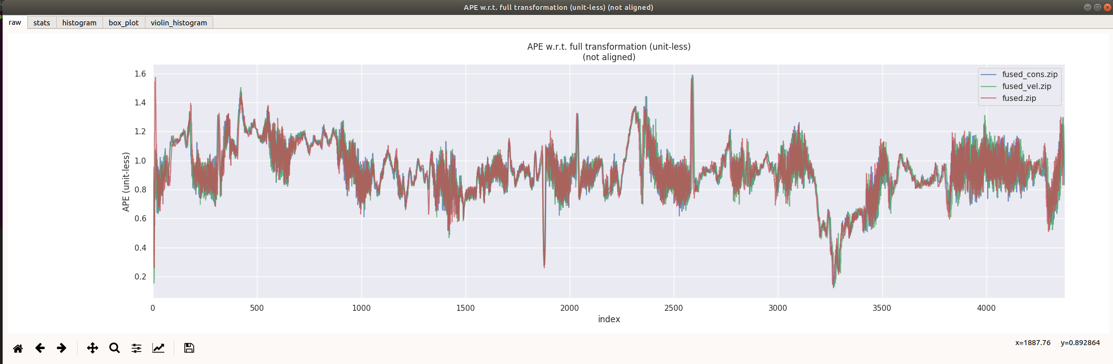
By observing the ape curve, I think there is not much difference
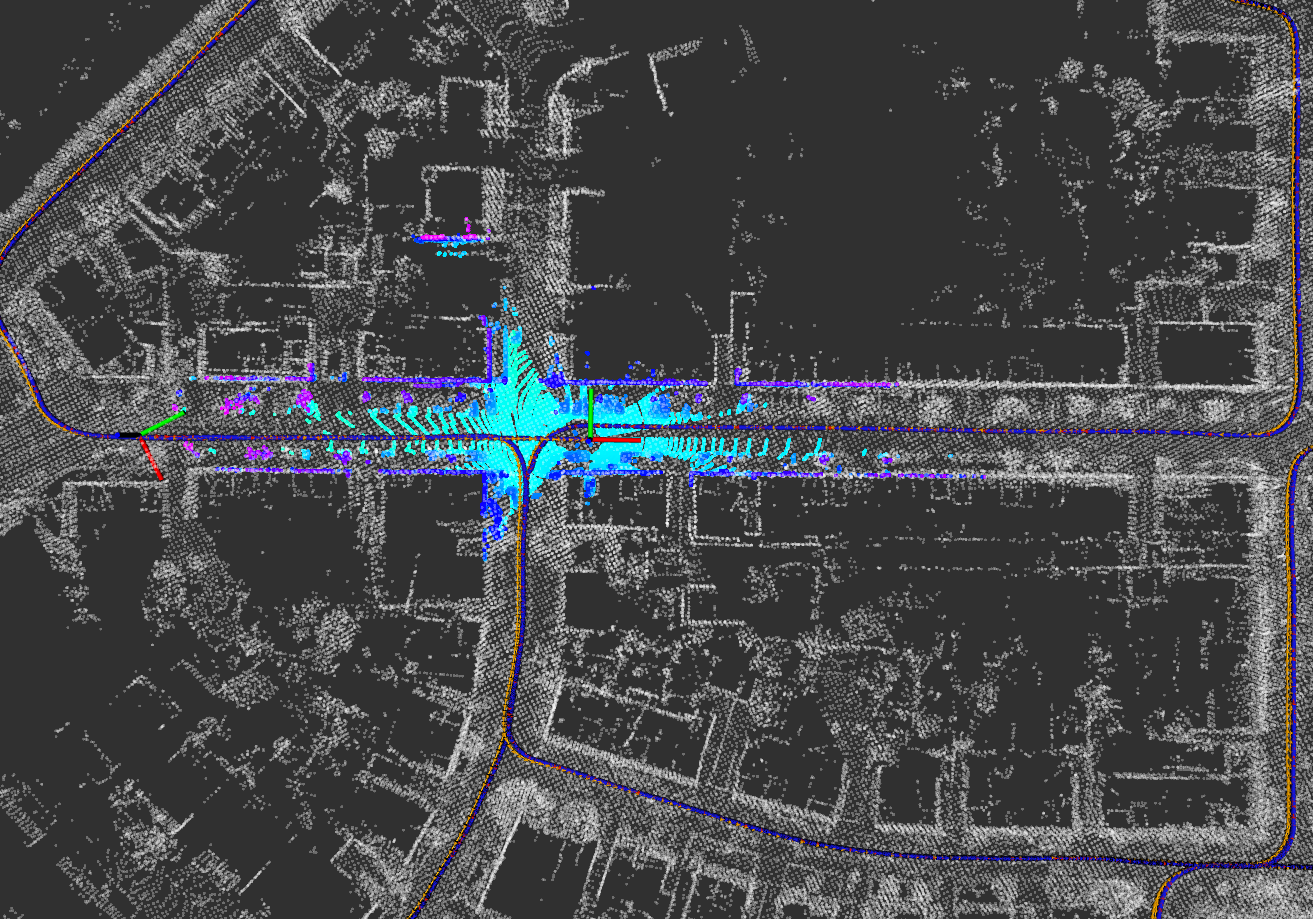
| fused no motion constraint | fused_cons motion constraint |
|---|---|
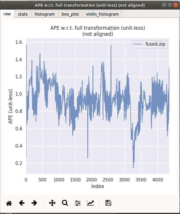 | 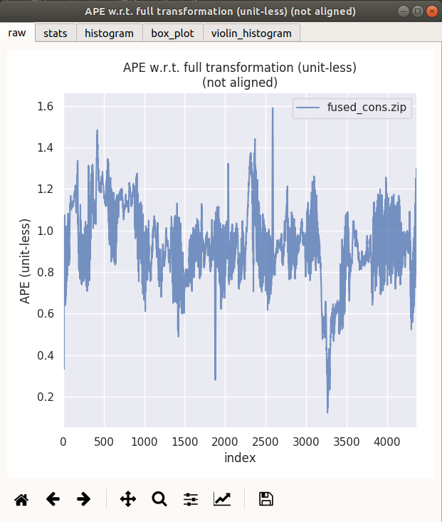 |
2.4.2 vel_y vel_z (body system) comparison after using the motion model
Fused means no motion constraint, fused_vel means adding inertial navigation velocity observation, and fused_cons means adding motion constraint (pseudo observation)
2.4.1 matplotlib visual data
To facilitate the visualization of v_x and v_z, matplotlib is used here to visualize the data
FILE: /home/kaho/shenlan_ws/visual/ main.py
# import necessary module
from mpl_toolkits.mplot3d import axes3d
import matplotlib.pyplot as plt
import numpy as np

fused = np.loadtxt("fused_withoust_cons.txt")
fused_vel_data = np.loadtxt("fused_vel.txt")
fused_cons_data = np.loadtxt("fused_cons.txt")

# x = fused_vel_data[:,0]
y_fused = fused[:,1]
z_fused = fused[:,2]

y_fused_vel = fused_vel_data[:,1]
z_fused_vel = fused_vel_data[:,2]

y_fused_cons_data = fused_cons_data[:,1]
z_fused_cons_data = fused_cons_data[:,2]

plt.plot(y_fused, c='r', label ="y_fused")
plt.plot(y_fused_vel, c='g', label ="Y_fused_vel")
# plt.plot(y_fused_cons_data, c='b', label ="y_fused_cons")
plt.legend();
plt.title('y velocity ',fontsize=18,color='y')
plt.show()

plt.plot(z_fused, c='r', label ="z_fused")
# plt.plot(z_fused_vel, c='g', label ="z_fused_vel")
plt.plot(y_fused_cons_data, c='b', label ="y_fused_cons")
plt.legend();
plt.title('z velocity ',fontsize=18,color='y')
plt.show()
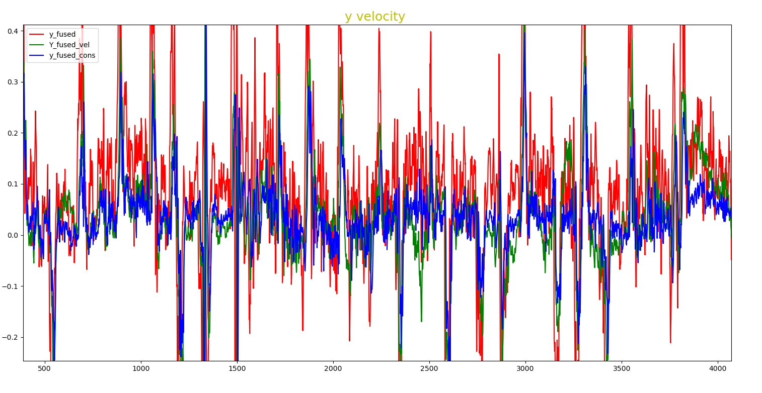
2.4.2 vel_y comparison
Red means no motion constraint, green means fused, speed observation is added, and blue means fused_cons means motion constraint is added. It can be clearly seen that the blue curve is under the red curve most of the time, indicating that the data volatility is less after using motion constraint.
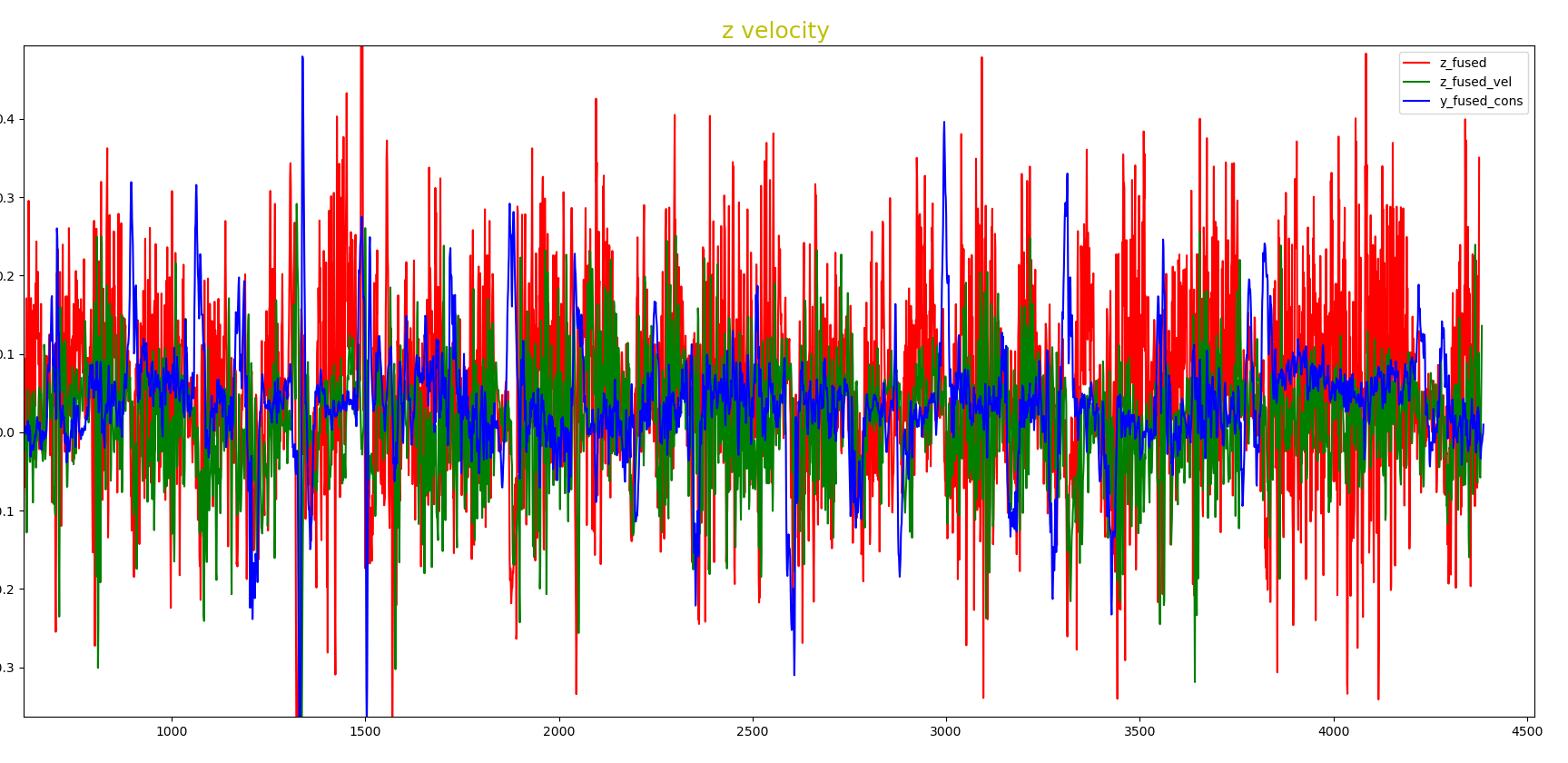
2.4.3 vel_z comparison
Red means no motion constraint, green means fused, speed observation is added, and blue means fused_cons means motion constraint is added. It can be clearly seen that the blue curve is under the red curve most of the time, indicating that the data volatility is less after using motion constraint.
2.4.4 conclusion
The experimental results are roughly consistent with the theory. After adding the motion model, the overall effect has been slightly improved, but the fluctuation of speed has been greatly restrained!!!
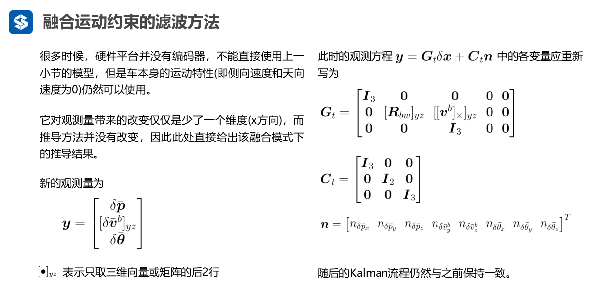
3. GNSS + Oodm observation model
Referring to the (estimate: IMU, measurement: lidar, odom) model, the (estimate: IMU, measurement: gnss, odom) model is derived. In the observation equation, gnss provides position and odom
3.1 formula derivation
State quantity
δ
x
=
[
δ
p
δ
v
δ
θ
δ
b
a
δ
b
ω
]
\delta \boldsymbol{x}=\left[\begin{array}{l} \delta \boldsymbol{p} \\ \delta \boldsymbol{v} \\ \delta \boldsymbol{\theta} \\ \delta \boldsymbol{b}_{a} \\ \delta \boldsymbol{b}_{\omega} \end{array}\right]
δx=⎣⎢⎢⎢⎢⎡δpδvδθδbaδbω⎦⎥⎥⎥⎥⎤
Observation GPS + Encoder for observation, GPS provides position and Encoder provides velocity
y
=
[
δ
p
‾
δ
v
‾
b
]
\boldsymbol{y}=\left[\begin{array}{c} \delta \overline{\boldsymbol{p}} \\ \delta \overline{\boldsymbol{v}}^{b} \\ \end{array}\right]
y=[δpδvb]
Acquisition of observations
δ
v
‾
b
=
v
~
b
−
v
b
=
R
~
b
w
v
~
w
−
[
v
m
0
0
]
\delta \overline{\boldsymbol{v}}_{b}=\tilde{\boldsymbol{v}}^{b}-\boldsymbol{v}^{b}=\tilde{\boldsymbol{R}}_{b w} \tilde{\boldsymbol{v}}^{w}-\left[\begin{array}{c} \boldsymbol{v}_{m} \\ 0 \\ 0 \end{array}\right]
δvb=v~b−vb=R~bwv~w−⎣⎡vm00⎦⎤
Observation equation
y
=
G
t
δ
x
+
C
t
n
\boldsymbol{y}=\boldsymbol{G}_{t} \delta \boldsymbol{x}+\boldsymbol{C}_{t} \boldsymbol{n}
y=Gtδx+Ctn
G t = [ I 3 0 0 0 0 0 R b w [ v b ] × 0 0 ] C t = [ I 3 0 0 I 3 ] \begin{aligned} \boldsymbol{G}_{t} &=\left[\begin{array}{ccccc} \boldsymbol{I}_{3} & \mathbf{0} & \mathbf{0} & \mathbf{0} & \mathbf{0} \\ \mathbf{0} & \boldsymbol{R}_{b w} & {\left[\boldsymbol{v}^{b}\right]_{\times}} & \mathbf{0} & \mathbf{0} \\ \end{array}\right] \\\\\\ \boldsymbol{C}_{t} &=\left[\begin{array}{ccc} \boldsymbol{I}_{3} & \mathbf{0} \\ \mathbf{0} & \boldsymbol{I}_{3} \\ \end{array}\right] \end{aligned} GtCt=[I300Rbw0[vb]×0000]=[I300I3]
n = [ n δ p ˉ x n δ p ˉ y n δ p ˉ z n δ v ˉ x b n δ v ˉ y b n δ v ˉ z b ] T \boldsymbol{n}=\left[\begin{array}{lllllllll} n_{\delta \bar{p}_{x}} & n_{\delta \bar{p}_{y}} & n_{\delta \bar{p}_{z}} & n_{\delta \bar{v}_{x}^{b}} & n_{\delta \bar{v}_{y}^{b}} & n_{\delta \bar{v}_{z}^{b}} \end{array}\right]^{T} n=[nδpˉxnδpˉynδpˉznδvˉxbnδvˉybnδvˉzb]T
3.2 correcterrorrestimationposivel, because the observation of ori is missing, the observation of orii can be deleted from the observation of (lidar + encoder).
void ErrorStateKalmanFilter::CorrectErrorEstimationPosiVel(       //  position + velocity
    const Eigen::Matrix4d &T_nb, const Eigen::Vector3d &v_b, const Eigen::Vector3d &w_b,
    Eigen::VectorXd &Y, Eigen::MatrixXd &G, Eigen::MatrixXd &K
) {
    //
    // TODO: set measurement: calculate the observed delta pos and delta velocity
    //
    Eigen::Vector3d  v_b_  =  {v_b[0],  0,  0};           //  Measurement velocity (body system), pseudo observation (vy, VZ = 0)

    Eigen::Vector3d  dp  =  pose_.block<3,  1>(0,  3)  -   T_nb.block<3,  1>(0,  3);
    Eigen::Vector3d  dv  =   pose_.block<3,  3>(0, 0).transpose() *vel_  -  v_b ;                  //  Delta V, v_x from wheel speed odometer
    // TODO: set measurement equation:
    YPosiVel_.block<3, 1>(0, 0)  =  dp;          //    delta  position
    YPosiVel_.block<3, 1>(3, 0)  =  dv;           //   delta   velocity
    Y = YPosiVel_;
    //   set measurement  G
    GPosiVel_.setZero();
    GPosiVel_.block<3, 3>(0, kIndexErrorPos)  =  Eigen::Matrix3d::Identity();
    GPosiVel_.block<3, 3>(3, kIndexErrorVel)   =   pose_.block<3,  3>(0, 0).transpose();
    GPosiVel_.block<3, 3>(3, kIndexErrorOri)   =   Sophus::SO3d::hat( pose_.block<3,  3>(0, 0).transpose() *vel_  ) ;
    G  =   GPosiVel_;
    //   set measurement  C
    CPosiVel_.setIdentity();
    Eigen::MatrixXd  C  =   CPosiVel_;
    // TODO: set Kalman gain:
    Eigen::MatrixXd R = RPosiVel_;    //  Observation noise
    K =  P_  *  G.transpose() * ( G  *  P_  *  G.transpose( )  +  C * R*  C.transpose() ).inverse() ;
}
3.3 parameter adjustment and gravity parameter modification
3.3.1 adjustment of POS vel observation error parameters
FILE: catkin_ws/src/lidar_localization/config/filtering/gnss_ins_sim_filtering.yaml
According to ta GeYao,
Finally, we need to remind you when running here, The two pictures on the left are gnss-ins-sim Error level when generating measurement data, Medium precision is used by default in the course, in other words gps The covariance of the position should be 2.5e-1 about, The encoder should be at 2.5e-3 about, On the right is the error level in the default configuration file used by our job. It can be seen that gps The difference between the actual error and the a priori value given by us is huge, That's why some students have the right program rviz The reason for the severe attitude jitter shown in. It is recommended that you adjust parameters based on the two values on the left.
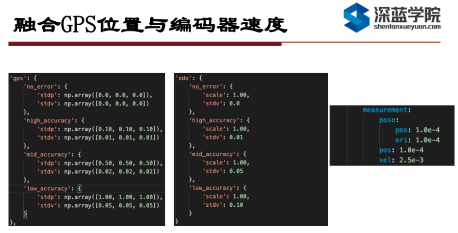
Therefore, we adjust the measurement cov of pos and vel to
        measurement:
            pose:
                pos: 1.0e-4
                ori: 1.0e-4
            pos: 2.5e-1 # 1.0-4
            vel: 2.5e-3
3.3.2 adjustment of gravity parameters
The gravity acceleration of the simulation data generated here is not consistent with that of kitti. The reason is that the positive direction of the Z axis of the sensor in the simulation data set is upward, so imu_sim_ins accel_z reads - g. By command rqt_bag checks the gravity acceleration read by the sensor and writes it to yaml.
FILE: catkin_ws/src/lidar_localization/config/filtering/gnss_ins_sim_filtering.yaml
gravity_magnitude: -9.794216
3.3.3 evo assessment
# set up session:
source devel/setup.bash
# save odometry:
rosservice call /save_odometry "{}"
# run evo evaluation:
# a. fused does not input the motion model, outputs the evaluation results, and stores them in zip format:
evo_ape kitti ground_truth.txt fused.txt -r full --plot --plot_mode xyz  --save_results ./fused.zip
# b. fused_vel velocity observation outputs the evaluation results and stores them in zip format:
evo_ape kitti ground_truth.txt gnss.txt -r full --plot --plot_mode xyz  --save_results ./gnss.zip
#e. Compare laser fused and evaluate together
evo_res  *.zip --use_filenames -p
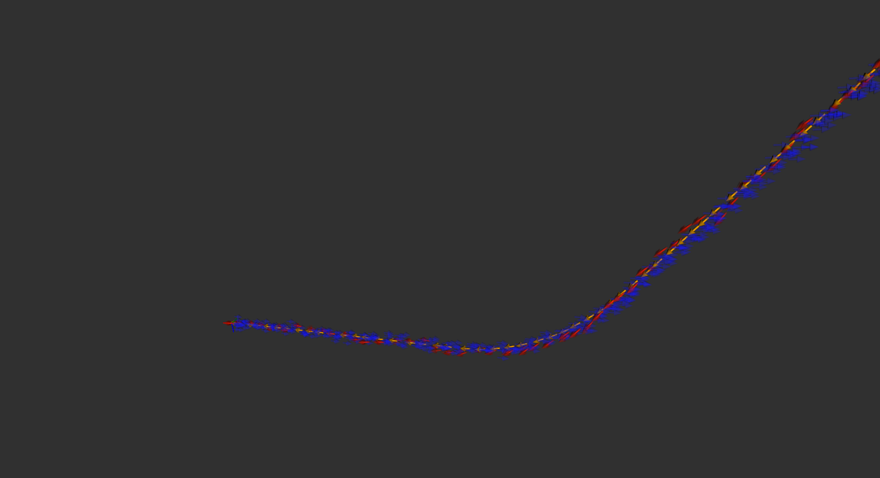
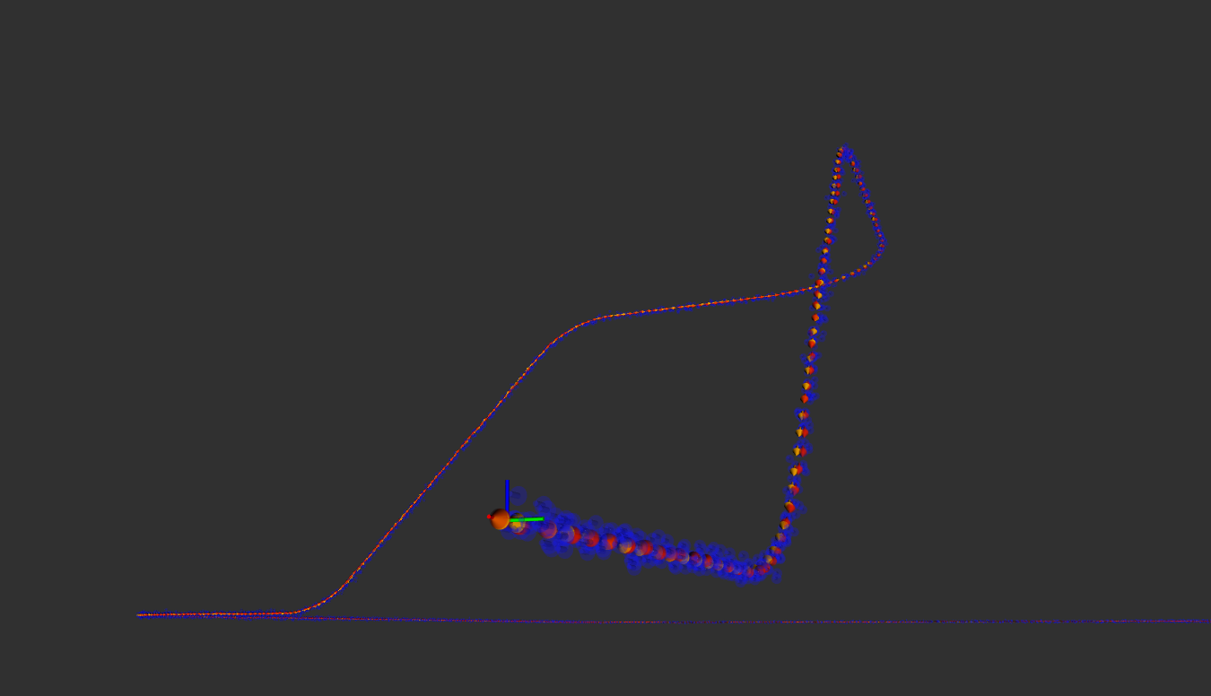
| GNSS + Odom | GNSS Only |
|---|---|
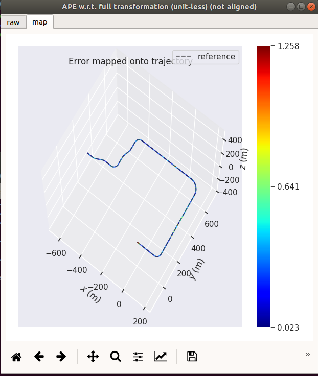 | 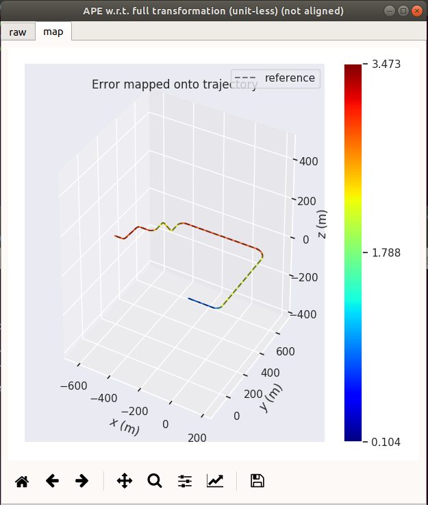 |
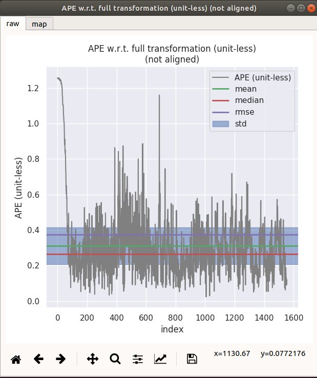 | 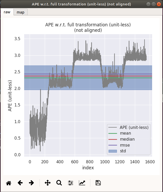 |
| max | mean | median | min | rmse | sse | std | |
|---|---|---|---|---|---|---|---|
| gnss+odom | 1.25794 | 0.31052 | 0.263991 | 0.0234911 | 0.374327 | 218.028 | 0.209041 |
| gnss only | 3.473 | 2.32244 | 2.37926 | 0.103637 | 2.43563 | 9230.62 | 0.733851 |
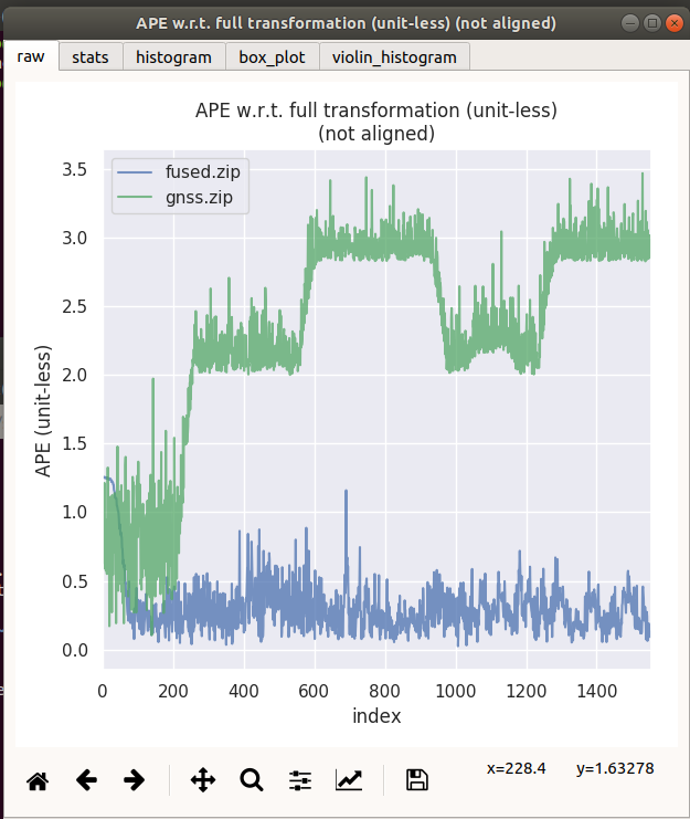
3.4 conclusion by comparing the above experiments
It can be seen that after the integration of odom wheel speed odometer, the data fluctuation is greatly suppressed.
edit by kaho 2021.10.22