Please note before reading:
1. MATLAB in-depth learning is an in-depth learning based on MATLAB learning notes. Learning this part requires a solid foundation of MATLAB. It is not recommended to learn this content without mastering the basic knowledge. The content of the blog is written and edited by @ K2SO4 potassium and published in the personal contribution of @ K2SO4 potassium and the official account of CSDN of HelloWorld programming Association of central China Normal University @ CCNU_HelloWorld . Note that if you need to reprint, you need the consent and authorization of the author @ K2SO4 potassium!
2. The codes and examples in the content are original by the author, and the references and other non original contents in the content will be marked at the end of the text in the form of references.
3. The example in the notes is MATLAB R2019a.
4. Please understand the possible errors in the notes and welcome correction and discussion; If the old code cannot be used due to MATLAB update, you are also welcome to discuss and exchange.
S6.0 MATLAB learning notes: portal summary
S6.0.1 MATLAB learning notes: portal summary
MATLAB learning notes 0: learning instructions
Matlab learning notes 1: overview of MATLAB
Matlab learning notes 2: basic knowledge of MATLAB (I)
Matlab learning notes 3: Fundamentals of MATLAB programming (first half)
Matlab learning notes 3: Fundamentals of MATLAB programming (second half)
S6.0.2 MATLAB extended learning: portal summary
MATLAB extended learning T1: anonymous functions and inline functions
MATLAB extended learning T2: program performance optimization technology
MATLAB extended learning T3: detailed explanation of histogram function
MATLAB extended learning T4: data import and table lookup Technology
S6.0.3 MATLAB in-depth learning: portal summary
In depth study of MATLAB S1: matlab implementation of simple digital filtering technology (1)
MATLAB in-depth study S2: infinite impulse response digital filter
MATLAB in-depth study S3: MATLAB implementation of simple digital filtering technology
In depth study of S4: cellular automata principle and MATLAB implementation
MATLAB in-depth study S5: image processing technology
S6: digital control technology -- interpolation principle of point by point comparison method
S6.0.4 MATLAB application example: portal summary
MATLAB application example Y1: Floyd algorithm
S6.1 point by point comparison straight line interpolation
Because our mechanical arm, cutter or painting pen are often controlled by the motor, and the direction of motor control is limited (generally speaking, it is the horizontal axis direction and vertical axis direction in the two-dimensional plane, and the z-axis direction needs to be considered in the three-dimensional plane. This paper only analyzes the horizontal and vertical direction in the two-dimensional plane), for some "walking obliquely" or "moving in an arc", The mechanical arm, cutting tool or painting pen controlled by motor can not move in the way of track accurately.
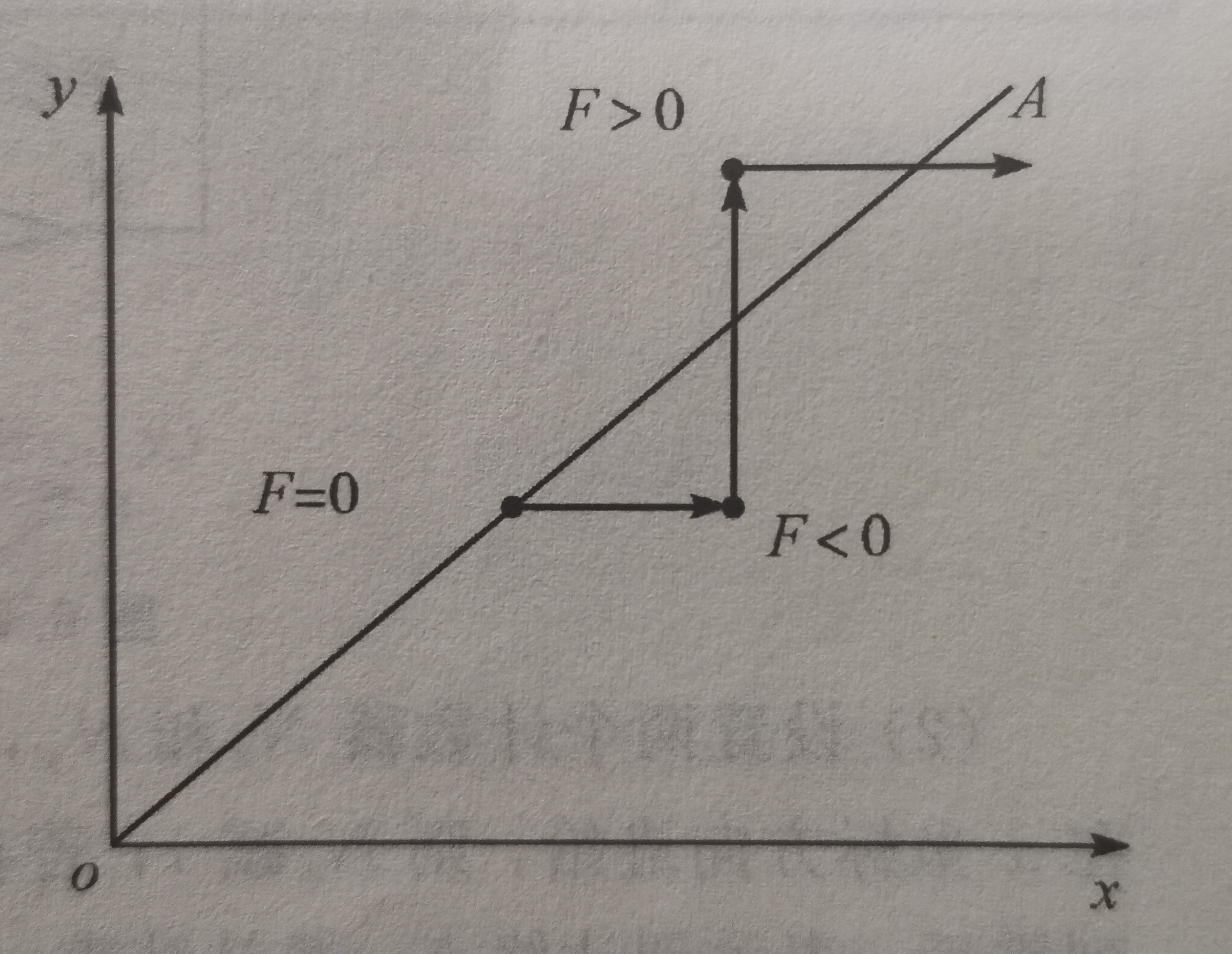
Point by point comparison interpolation is actually well understood. It is to compare the current position of the tool with the given trajectory (or ideal trajectory), and see whether the current point is above or below the trajectory, inside or outside the trajectory, so as to determine whether the next step is horizontal or vertical. Whether moving horizontally or vertically, there will be a "step", that is, the minimum value of movement, and all moving distances are multiples of it. When the step size is very small, the point by point comparison method can be used for interpolation, and the tool can be moved more accurately for the linear path in any direction.
For a curve, with the idea of calculus, we can divide a curve into several straight lines. Carry out the above method for each straight line, and then combine the expected operation mode of each straight line tool, and finally the expected movement path of the tool on the whole curve. Of course, if the curve is divided into straight lines "too thin", it will lead to too long code running time, too much storage and high cost. Therefore, for the curve, if the accuracy requirement is high, the straight-line interpolation of point by point comparison method is not applicable.
After talking about the general principle, let's talk about the details:
(1) The linear interpolation methods in different quadrants are slightly different
Rather than "straight lines in different quadrants", it is more accurate to say the direction from the starting point to the end point. After determining the direction from the start point to the end point:
If the direction is the positive direction of the first quadrant or horizontal axis:
If the current point of the tool is on or above the track, the tool should step to the right;
If the current point of the tool is below the track, the tool should step up;
If the direction is the second quadrant or the negative direction of the horizontal axis:
If the current point of the tool is on or above the track, the tool should step to the left;
If the current point of the tool is below the track, the tool should step up;
If the direction is the third quadrant:
If the current point of the tool is on or below the track, the tool should step to the left;
If the current point of the tool is above the track, the tool should step down;
If the direction is the fourth quadrant:
If the current point of the tool is on or below the track, the tool should step to the right;
If the current point of the tool is above the track, the tool should step down;
If the direction is the positive or negative direction of the longitudinal axis
Tool up or down step
(2) When is the end of the run
When the tool falls in the end coordinate range ( step enter long degree ) / 2 (step length) / 2 Above or within (step length) / 2, it can be considered that the tool movement is over.
(3) When taking the curve as the ideal trajectory
When taking the curve as the ideal track, it should be noted that there should not be too many lines to segment, otherwise the running cost is too large. Secondly, when synthesizing the tool movement tracks recorded by all straight lines, it is necessary to delete the repeated points in the two tracks.
The following are the integrated functions and test procedures. (there is a slight problem with this function, which will be fixed in subsequent updates, but the principle is correct)
function [res_x,res_y] = PBPC_Linear_Interpolation(start_x,start_y,current_x,current_y,end_x,end_y,step_x,step_y)
%
% Take step_x and step_y as the step values in the horizontal and vertical directions,
% then use the point by point comparison method to return the linear interpolation
% from point (start_x, start_y) to point (end_x, end_y)
%
% with step_x,step_y Is the step value in the horizontal and vertical direction, and the point by point comparison method returns the slave point(start_x,start_y)To point(end_x,end_y)Linear interpolation
%
% input parameter (start_x, start_y): Abscissa and ordinate of starting point
% input parameter (end_x, end_y): End point abscissa and ordinate
% input parameter (current_x,current_y): The current position of the tool or pen drawing
% Output parameters step_x,step_y: Step value of tool or pen drawing
% Output parameters(res_x,res_y): Tool or pen trace
%
% Common calling methods:
% [res_x,res_y] = PBPC_Linear_Interpolation(start_x,start_y,current_x,current_y,end_x,end_y,step_x,step_y)
%
% Prepared on October 19, 2021:26   programmer: K2SO4 potassium
%

if start_x == end_x
    res_x = [];
    res_y = [];
    res_x(1) = start_x;
    res_y(1) = start_y;

    counter = 2;
    if end_y >= start_y
        while(1)
            if current_x >= end_x-step_x/2 && current_x <= end_x+step_x/2 && ...
                    current_y >= end_y-step_y/2 && current_y <= end_y+step_y/2
                break
            end
            current_y = current_y+step_y;
            res_x(1,counter) = current_x;
            res_y(1,counter) = current_y;
            counter = counter+1;
        end
    else
        while(1)
            if current_x >= end_x-step_x/2 && current_x <= end_x+step_x/2 && ...
                    current_y >= end_y-step_y/2 && current_y <= end_y+step_y/2
                break
            end
            current_y = current_y-step_y;
            res_x(1,counter) = current_x;
            res_y(1,counter) = current_y;
            counter = counter+1;
        end
    end
end

if start_y == end_y
    res_x = [];
    res_y = [];
    res_x(1) = start_x;
    res_y(1) = start_y;

    counter = 2;
    if end_x >= start_x
        while(1)
            if current_x >= end_x-step_x/2 && current_x <= end_x+step_x/2 && ...
                    current_y >= end_y-step_y/2 && current_y <= end_y+step_y/2
                break
            end
            current_x = current_x+step_x;
            res_x(1,counter) = current_x;
            res_y(1,counter) = current_y;
            counter = counter+1;
        end
    else
        while(1)
            if current_x >= end_x-step_x/2 && current_x <= end_x+step_x/2 && ...
                    current_y >= end_y-step_y/2 && current_y <= end_y+step_y/2
                break
            end
            current_x = current_x-step_x;
            res_x(1,counter) = current_x;
            res_y(1,counter) = current_y;
            counter = counter+1;
        end
    end
end

if start_x ~= end_x
    k = (start_y-end_y)/(start_x-end_x);
    x0 = start_x;
    y0 = start_y;
    syms x
    func = matlabFunction(k*(x-x0)+y0);

    res_x = [];
    res_y = [];
    res_x(1) = start_x;
    res_y(1) = start_y;

    counter = 2;
    if end_x > start_x && end_y >= start_y
        while(1)
            if current_x >= end_x-step_x/2 && current_x <= end_x+step_x/2 && ...
                    current_y >= end_y-step_y/2 && current_y <= end_y+step_y/2
                break
            end
            if current_y >= func(current_x)
                current_x = current_x+step_x;
                res_x(1,counter) = current_x;
                res_y(1,counter) = current_y;
                counter = counter+1;
            else
                current_y = current_y+step_y;
                res_x(1,counter) = current_x;
                res_y(1,counter) = current_y;
                counter = counter+1;
            end
        end
    elseif end_x < start_x && end_y >= start_y
        while(1)
            if current_x >= end_x-step_x/2 && current_x <= end_x+step_x/2 && ...
                    current_y >= end_y-step_y/2 && current_y <= end_y+step_y/2
                break
            end
            if current_y >= func(current_x)
                current_x = current_x-step_x;
                res_x(1,counter) = current_x;
                res_y(1,counter) = current_y;
                counter = counter+1;
            else
                current_y = current_y+step_y;
                res_x(1,counter) = current_x;
                res_y(1,counter) = current_y;
                counter = counter+1;
            end
        end
    elseif end_x > start_x && end_y < start_y
        while(1)
            if current_x >= end_x-step_x/2 && current_x <= end_x+step_x/2 && ...
                    current_y >= end_y-step_y/2 && current_y <= end_y+step_y/2
                break
            end
            if current_y <= func(current_x)
                current_x = current_x+step_x;
                res_x(1,counter) = current_x;
                res_y(1,counter) = current_y;
                counter = counter+1;
            else
                current_y = current_y-step_y;
                res_x(1,counter) = current_x;
                res_y(1,counter) = current_y;
                counter = counter+1;
            end
        end
    elseif end_x < start_x && end_y < start_y
         while(1)
             if current_x >= end_x-step_x/2 && current_x <= end_x+step_x/2 && ...
                    current_y >= end_y-step_y/2 && current_y <= end_y+step_y/2
                break
            end
            if current_y <= func(current_x)
                current_x = current_x-step_x;
                res_x(1,counter) = current_x;
                res_y(1,counter) = current_y;
                counter = counter+1;
            else
                current_y = current_y-step_y;
                res_x(1,counter) = current_x;
                res_y(1,counter) = current_y;
                counter = counter+1;
            end
         end
    end
end

end
%% simulation
clc,clear all,close all

start_x = 0;
start_y = 3;
end_x = 16;
end_y = 18;
[X,Y] = PBPC_Linear_Interpolation(start_x,start_y,start_x,start_y,end_x,end_y,0.6,0.8);
subplot(121)
plot(X,Y,'linewidth',1.4)
hold on
line([start_x,end_x],[start_y,end_y],'color','r','linewidth',1.4)
title('Image 1')

start_x = 0;
start_y = 3;
end_x = 120;
end_y = 140;
[X,Y] = PBPC_Linear_Interpolation(start_x,start_y,start_x,start_y,end_x,end_y,0.1,0.1);
subplot(122)
plot(X,Y,'linewidth',1.4)
hold on
line([start_x,end_x],[start_y,end_y],'color','r','linewidth',1.4)
title('Image 2')
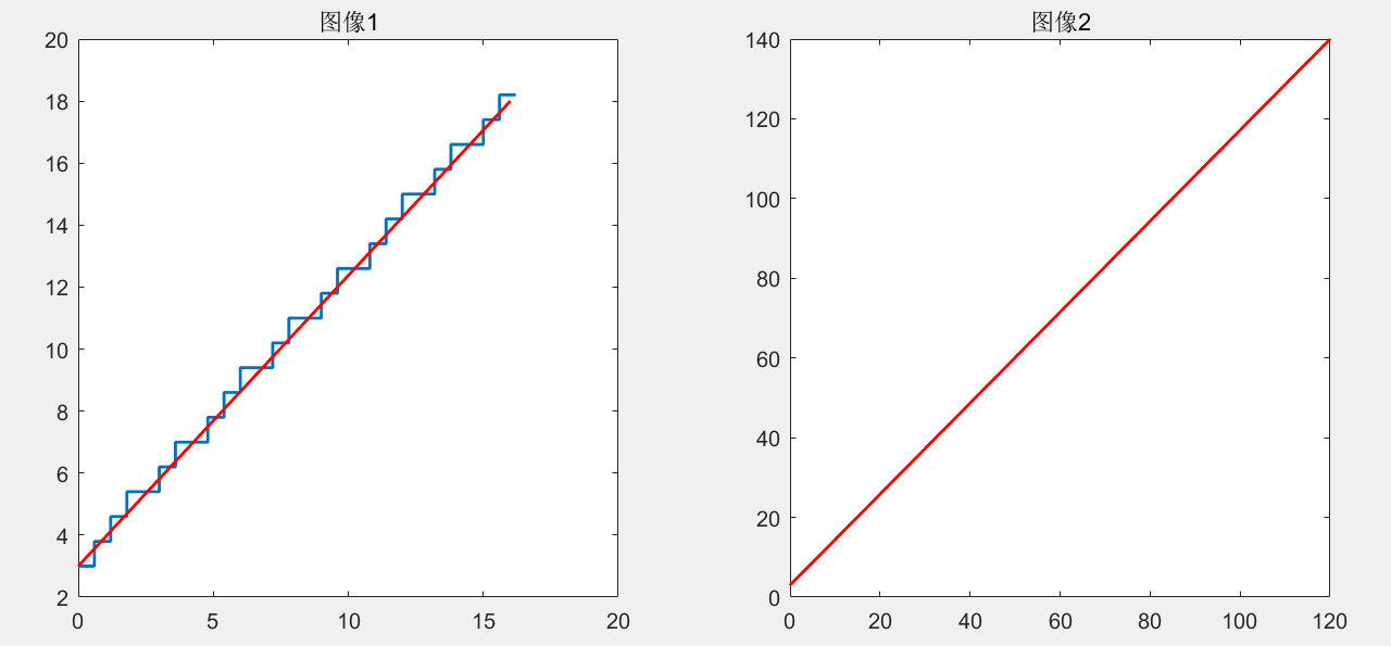
When the step is very small, the moving path of the tool almost coincides with the ideal path (as shown in the right figure).
Author: K2SO4 potassium (Central China Normal University)