1 Preface

Hi, Hello, this is Dancheng, and today we introduce the classification of breast cancer based on convolution neural network.

This is the subject of deep learning in medical image classification

You can use it for graduation design

Bi design help, problem opening guidance, technical solutions
🇶746876041

2 PREFACE

Breast cancer is the second most common cancer in the world. In 2012, it accounted for 12% of all new cancer cases and 25% of all female cancer cases.

When breast cells grow out of control, breast cancer begins. These cells usually form a tumor, and a mass can usually be seen or felt directly on the x-ray film. If cancer cells can grow into surrounding tissues or spread to other parts of the body, the tumor is malignant.

The following is the report:

• About 1/8 of American women (about 12%) will develop invasive breast cancer in their lifetime.
• In 2019, the United States is expected to have 268600 cases of new invasive breast cancer and 62930 cases of new non-invasive breast cancer.
• About 85% of breast cancer occurs in women without family history of breast cancer. These occur because of genetic mutations, not genetic mutations
• If a woman's first degree relatives (mother, sister, daughter) are diagnosed with breast cancer, the risk of breast cancer will almost double. Less than 15% of the women who have breast cancer are diagnosed with breast cancer.

3 data set

The data set is the senior laboratory data set.

First, this is the problem of image classification. I split the data as shown in the figure

dataset train
  benign
   b1.jpg
   b2.jpg
   //
  malignant
   m1.jpg
   m2.jpg
   //  validation
   benign
    b1.jpg
    b2.jpg
    //
   malignant
    m1.jpg
    m2.jpg
    //...

The training folder has 1000 images in each category, while the validation folder has 250 images in each category.

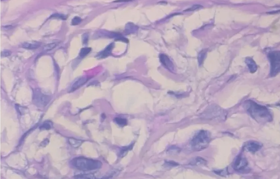
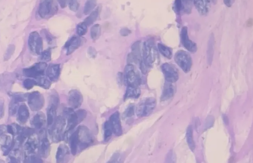
3.1 benign samples

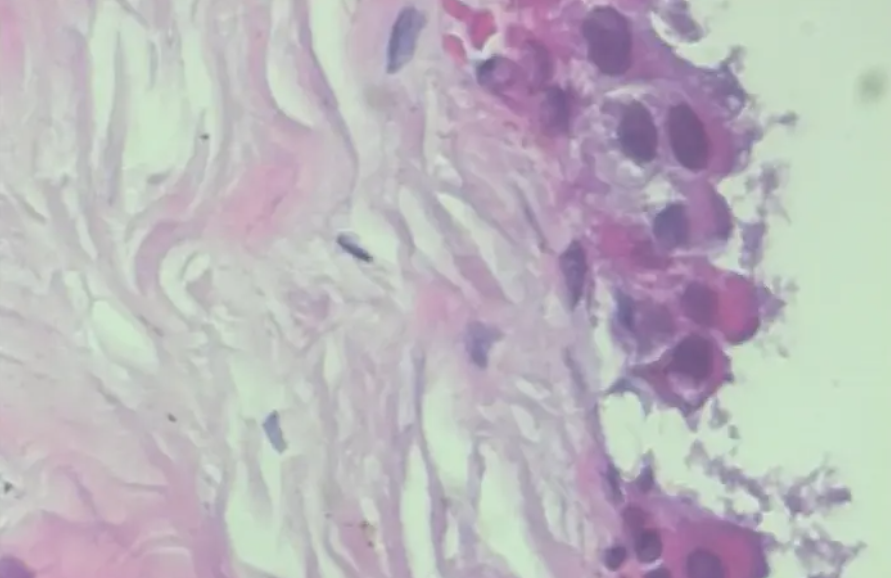
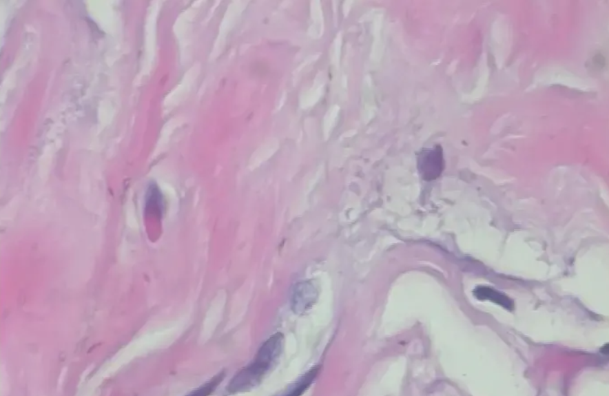
3.2 lesion samples

4 development environment

• scikit-learn
• keras
• numpy
• pandas
• matplotlib
• tensorflow

5 code implementation

5.1 implementation process

The complete image classification process can be formalized as follows:

Our input is a training data set composed of N images, and each image has a corresponding label.

Then, we use this training set to train the classifier to learn each class.

Finally, we evaluate the quality of the classifier by asking the classifier to predict the labels of a set of new images we have never seen before. Then we compare the real tags of these images with the tags predicted by the classifier.

5.2 partial code implementation

5.2.1 import and stock in

import json
import math
import os
import cv2
from PIL import Image
import numpy as np
from keras import layers
from keras.applications import DenseNet201
from keras.callbacks import Callback, ModelCheckpoint, ReduceLROnPlateau, TensorBoard
from keras.preprocessing.image import ImageDataGenerator
from keras.utils.np_utils import to_categorical
from keras.models import Sequential
from keras.optimizers import Adam
import matplotlib.pyplot as plt
import pandas as pd
from sklearn.model_selection import train_test_split
from sklearn.metrics import cohen_kappa_score, accuracy_score
import scipy
from tqdm import tqdm
import tensorflow as tf
from keras import backend as K
import gc
from functools import partial
from sklearn import metrics
from collections import Counter
import json
import itertools

5.2.2 image loading

Next, I load the image into the corresponding folder.

def Dataset_loader(DIR, RESIZE, sigmaX=10):
    IMG = []
    read = lambda imname: np.asarray(Image.open(imname).convert("RGB"))
    for IMAGE_NAME in tqdm(os.listdir(DIR)):
        PATH = os.path.join(DIR,IMAGE_NAME)
        _, ftype = os.path.splitext(PATH)
        if ftype == ".png":
            img = read(PATH)
           
            img = cv2.resize(img, (RESIZE,RESIZE))
           
            IMG.append(np.array(img))
    return IMG

benign_train = np.array(Dataset_loader('data/train/benign',224))
malign_train = np.array(Dataset_loader('data/train/malignant',224))
benign_test = np.array(Dataset_loader('data/validation/benign',224))
malign_test = np.array(Dataset_loader('data/validation/malignant',224))

5.2.3 marking

After that, I created a numpy array of all zeros to mark benign images and a numpy array of all 1s to mark malignant images. I also reorganized the dataset and converted the labels to classification format.

benign_train_label = np.zeros(len(benign_train))
malign_train_label = np.ones(len(malign_train))
benign_test_label = np.zeros(len(benign_test))
malign_test_label = np.ones(len(malign_test))

X_train = np.concatenate((benign_train, malign_train), axis = 0)
Y_train = np.concatenate((benign_train_label, malign_train_label), axis = 0)
X_test = np.concatenate((benign_test, malign_test), axis = 0)
Y_test = np.concatenate((benign_test_label, malign_test_label), axis = 0)

s = np.arange(X_train.shape[0])
np.random.shuffle(s)
X_train = X_train[s]
Y_train = Y_train[s]

s = np.arange(X_test.shape[0])
np.random.shuffle(s)
X_test = X_test[s]
Y_test = Y_test[s]

Y_train = to_categorical(Y_train, num_classes= 2)
Y_test = to_categorical(Y_test, num_classes= 2)

5.2.4 grouping

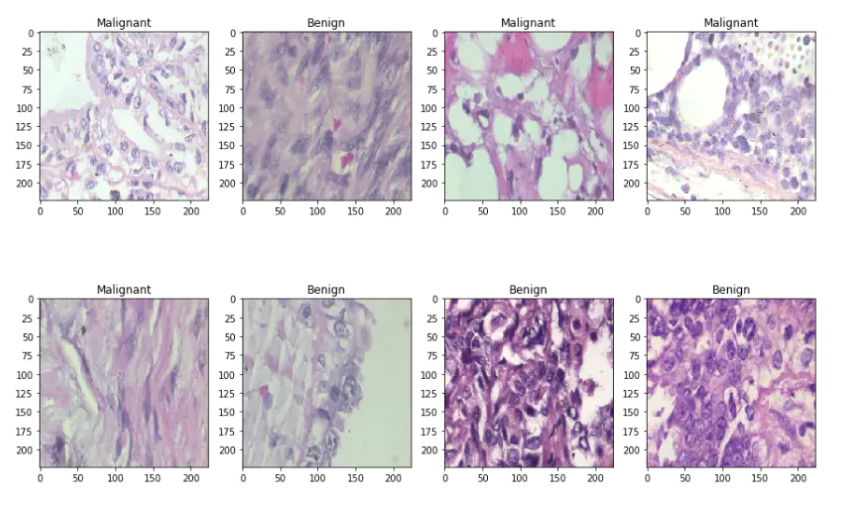
Then I divided the data set into two groups, training set and test set with 80% and 20% images respectively. Let's look at some samples of benign and malignant images

x_train, x_val, y_train, y_val = train_test_split(
    X_train, Y_train, 
    test_size=0.2, 
    random_state=11
)

w=60
h=40
fig=plt.figure(figsize=(15, 15))
columns = 4
rows = 3

for i in range(1, columns*rows +1):
    ax = fig.add_subplot(rows, columns, i)
    if np.argmax(Y_train[i]) == 0:
        ax.title.set_text('Benign')
    else:
        ax.title.set_text('Malignant')
    plt.imshow(x_train[i], interpolation='nearest')
plt.show()

5.2.5 model building training

I used a batch value of 16. Batch is one of the most important super parameters in deep learning. I prefer to use a larger batch to train my model because it allows to improve the computing speed from the parallelism of gpu. However, as we all know, batch is too large, resulting in poor generalization effect. At one extreme, using a batch equal to the entire data set will ensure convergence to the global optimization of the objective function. But this is at the cost of slow convergence to the optimal value. On the other hand, using smaller batch has been proved to converge to good results faster. This can be explained intuitively that a smaller batch allows the model to start learning before it has to view all the data. The disadvantage of using smaller batch is that it can not guarantee that the model converges to the global optimum. Therefore, it is generally recommended to start from a small batch and slowly increase the batch size through training to speed up the convergence speed.

I also made some data expansion. The practice of data expansion is an effective way to increase the scale of training set. The expansion of training examples makes the network see more diversified and representative data points in the training process.

Then I created a data generator to automatically get data from folders. Keras provides a convenient python generator function for this purpose.

BATCH_SIZE = 16

train_generator = ImageDataGenerator(
        zoom_range=2,  # Set the range to random scaling
        rotation_range = 90,
        horizontal_flip=True,  # Randomly flip pictures
        vertical_flip=True,  # Randomly flip pictures
    )

The next step is to build the model. This can be described in the following three steps:

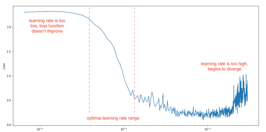
• I use DenseNet201 as the weight before training, which has been trained in the Imagenet competition. Set the learning rate to 0.0001.

• On this basis, I used the global average pooling layer and 50% dropout to reduce over fitting.

• I use batch standardization and a full connection layer with two neurons with softmax as the activation function for the benign and malignant of two output classes.

• I use Adam as the optimizer and binary cross entropy as the loss function.

def build_model(backbone, lr=1e-4):
    model = Sequential()
    model.add(backbone)
    model.add(layers.GlobalAveragePooling2D())
    model.add(layers.Dropout(0.5))
    model.add(layers.BatchNormalization())
    model.add(layers.Dense(2, activation='softmax'))
    
    model.compile(
        loss='binary_crossentropy',
        optimizer=Adam(lr=lr),
        metrics=['accuracy']
    )
    return model

resnet = DenseNet201(
    weights='imagenet',
    include_top=False,
    input_shape=(224,224,3)
)

model = build_model(resnet ,lr = 1e-4)
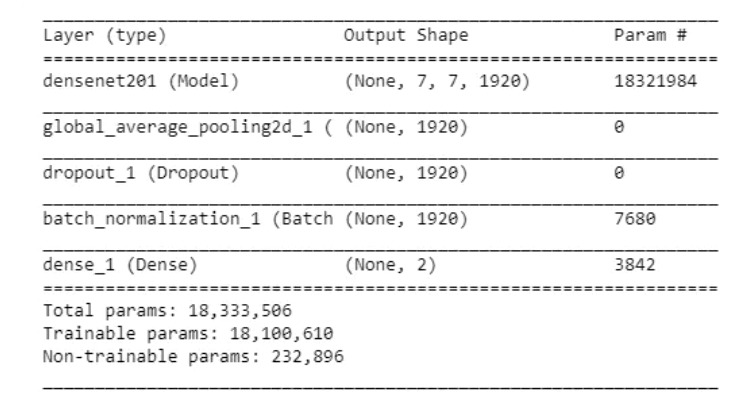
model.summary()

Let's look at the output shapes and parameters in each layer.

It is useful to define one or more callback functions before training the model. Very convenient: ModelCheckpoint and reducerlonplateau.

• ModelCheckpoint: when training usually requires multiple iterations and takes a lot of time to achieve a good result, ModelCheckpoint saves the best model in the training process.

• Reducerlonplateau: when the measurement stops improving, the learning rate is reduced. Once learning stagnates, the model usually reduces the learning rate by 2-10 times. This callback function will monitor. If the model is not optimized under the 'patience' times, the learning rate will be reduced.

I trained 60 epoch s in this model.

learn_control = ReduceLROnPlateau(monitor='val_acc', patience=5,
                                  verbose=1,factor=0.2, min_lr=1e-7)

filepath="weights.best.hdf5"
checkpoint = ModelCheckpoint(filepath, monitor='val_acc', verbose=1, save_best_only=True, mode='max')

history = model.fit_generator(
    train_generator.flow(x_train, y_train, batch_size=BATCH_SIZE),
    steps_per_epoch=x_train.shape[0] / BATCH_SIZE,
    epochs=20,
    validation_data=(x_val, y_val),
    callbacks=[learn_control, checkpoint]
)

6 Analysis Indicators

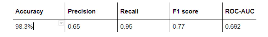
The most commonly used index to evaluate the performance of the model is accuracy. However, when only 2% of your dataset belongs to one class (malignant) and 98% to other classes (benign), the misclassification score is meaningless. You can have 98% accuracy, but still no malignant cases are found, that is, when predicting, all are labeled as benign, which is a bad classifier.

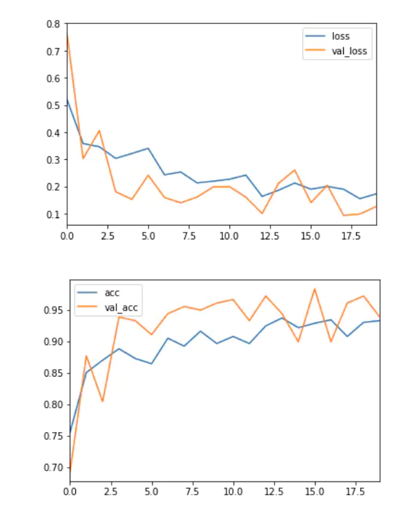
history_df = pd.DataFrame(history.history)
history_df[['loss', 'val_loss']].plot()

history_df = pd.DataFrame(history.history)
history_df[['acc', 'val_acc']].plot()

6.1 precision, recall and F1 metrics

To better understand misclassification, we often use the following metrics to better understand real cases (TP), true negative cases (TN), false positive cases (FP) and false negative cases (FN).

The accuracy reflects the proportion of real positive samples in the positive samples determined by the classifier.

The recall rate reflects the proportion of all samples that are really positive examples determined by the classifier as positive examples.

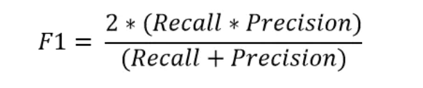
The F1 measure is the harmonic average of accuracy and recall.

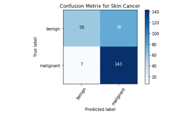
6.2 confusion matrix

Confusion matrix is an important index to analyze misclassification. Each row of the matrix represents instances in the predicted class, while each column represents instances in the actual class. Diagonals represent correctly classified classes. This is helpful because we know not only which classes are misclassified, but also why they are misclassified.

from sklearn.metrics import classification_report
classification_report( np.argmax(Y_test, axis=1), np.argmax(Y_pred_tta, axis=1))

from sklearn.metrics import confusion_matrix

def plot_confusion_matrix(cm, classes,
                          normalize=False,
                          title='Confusion matrix',
                          cmap=plt.cm.Blues):
    if normalize:
        cm = cm.astype('float') / cm.sum(axis=1)[:, np.newaxis]
        print("Normalized confusion matrix")
    else:
        print('Confusion matrix, without normalization')

    print(cm)

    plt.imshow(cm, interpolation='nearest', cmap=cmap)
    plt.title(title)
    plt.colorbar()
    tick_marks = np.arange(len(classes))
    plt.xticks(tick_marks, classes, rotation=55)
    plt.yticks(tick_marks, classes)
    fmt = '.2f' if normalize else 'd'
    thresh = cm.max() / 2.
    for i, j in itertools.product(range(cm.shape[0]), range(cm.shape[1])):
        plt.text(j, i, format(cm[i, j], fmt),
                 horizontalalignment="center",
                 color="white" if cm[i, j] > thresh else "black")

    plt.ylabel('True label')
    plt.xlabel('Predicted label')
    plt.tight_layout()

cm = confusion_matrix(np.argmax(Y_test, axis=1), np.argmax(Y_pred, axis=1))

cm_plot_label =['benign', 'malignant']
plot_confusion_matrix(cm, cm_plot_label, title ='Confusion Metrix for Skin Cancer')

7 results and conclusions

In this blog, I demonstrated how to use convolution neural network and transfer learning to classify benign and malignant breast cancer from a group of microscopic images.

8 finally - design help

Bi design help, problem opening guidance, technical solutions
🇶746876041