Activation function
Function of activation function
Real examples in life are very complex, and it is difficult to represent all the data with straight lines. In fact, real data is easier to represent with curves. Therefore, the activation function is introduced.
Classification of activation functions
The commonly used activation functions are Sigmoid, relu, tanh and leaky_relu.
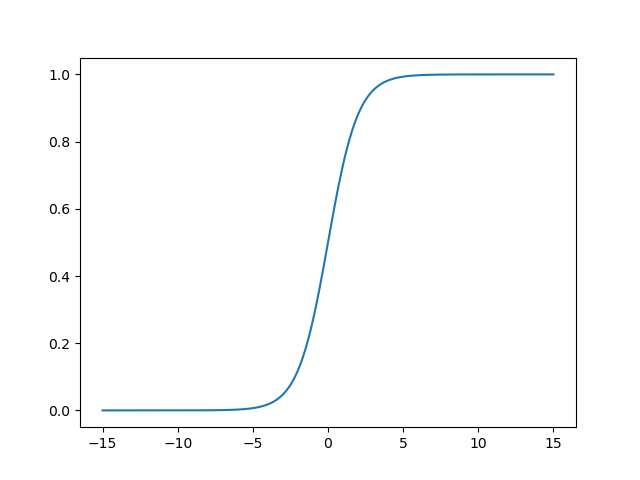
Sigmoid
S
i
g
m
o
i
d
(
x
)
=
1
1
+
e
−
x
Sigmoid(x)= \frac{1}{1+e^{-x}}
Sigmoid(x)=1+e−x1
∂
S
i
g
m
o
i
d
(
x
)
∂
x
=
S
i
g
m
o
i
d
(
x
)
∗
(
1
−
S
i
g
m
o
i
d
(
x
)
)
\frac{\partial{Sigmoid(x)}}{\partial{}x}=Sigmoid(x)*(1-Sigmoid(x))
∂x∂Sigmoid(x)=Sigmoid(x)∗(1−Sigmoid(x))
S
i
g
m
o
i
d
(
x
)
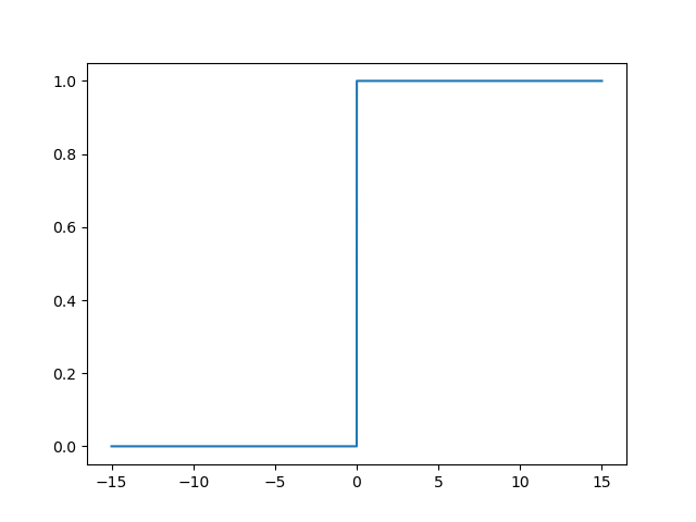
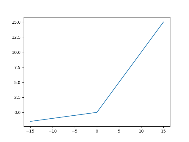
Sigmoid(x)
Sigmoid(x) function image
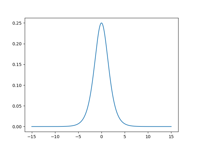
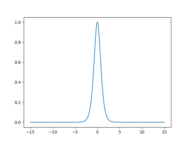
∂
S
i
g
m
o
i
d
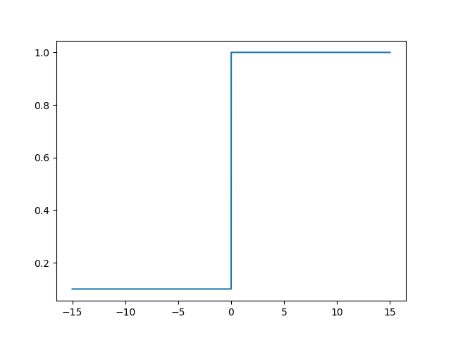
∂
x
\frac{\partial{Sigmoid}}{\partial{}x}
∂ x ∂ Sigmoid function image
The advantages of Sigmoid are:
- It can compress data to ensure that there is no problem with data amplitude.
- Smoothing function for easy derivation.
- Suitable for forward propagation.
The disadvantages of Sigmoid are:
- The phenomenon of gradient vanishing is easy to occur.
- The output of Sigmoid is not 0 mean, which makes the convergence slow.
- Power operation is relatively time-consuming.
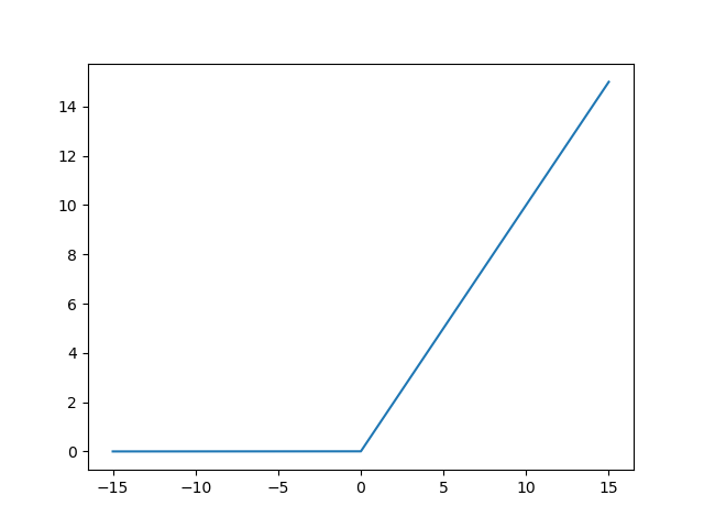
Relu
R
e
l
u
(
x
)
=
{
x
,
x>=0
0
,
x<0
Relu(x) = \begin{cases}x, & \text{x>=0} \\0, & \text{x<0} \end{cases}
Relu(x)={x,0,x>=0x<0
∂
R
e
l
u
(
x
)
∂
x
=
{
1
,
x>=0
0
,
x<0
\frac{\partial{Relu(x)}}{\partial{x}}=\begin{cases}1, & \text{x>=0} \\0, & \text{x<0} \end{cases}
∂x∂Relu(x)={1,0,x>=0x<0
R
e
l
u
(
x
)
Relu(x)
Function image of Relu(x)
∂
R
e
l
u
(
x
)
∂
x
\frac{\partial{Relu(x)}}{\partial{x}}
∂ x ∂ Relu(x) function image
 R
e
l
u
(
x
)
Relu(x)
The advantage of Relu(x) is
R
e
l
u
(
x
)
Relu(x)
The advantage of Relu(x) is
- The convergence rate of ReLu is faster than sigmoid and tanh.
- Suitable for backward propagation.
R e l u ( x ) Relu(x) The disadvantage of Relu(x) is
- The output of Relu is not 0 mean, which makes the convergence slow.
- Some neurons may never be activated, so that the corresponding parameters will never be updated.
- ReLU will not compress the data amplitude, so the data amplitude will continue to expand with the increase of the number of model layers.
Tanh
T
a
n
h
(
x
)
=
e
x
−
e
−
x
e
x
+
e
−
x
Tanh(x) = \frac{e^x-e^{-x}}{e^x+e^{-x}}
Tanh(x)=ex+e−xex−e−x
∂
T
a
n
h
(
x
)
∂
x
=
1
−
(
T
a
n
h
(
x
)
)
2
\frac{\partial{Tanh(x)}}{\partial{x}}=1-(Tanh(x))^2
∂x∂Tanh(x)=1−(Tanh(x))2
T
a
n
h
(
x
)
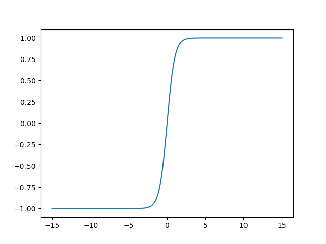
Tanh(x)
Tanh(x) function image
∂
T
a
n
h
(
x
)
∂
x
\frac{\partial{Tanh(x)}}{\partial{x}}
∂ x ∂ Tanh(x) function image
T
a
n
h
(
x
)
Tanh(x)
The advantage of Tanh(x) is
- Tanh function is 0 mean, which is more conducive to improve the training efficiency
T a n h ( x ) Tanh(x) The disadvantage of Tanh(x) is
- The problems of gradient vanishing and power operation still exist.
Leaky_relu
L
e
a
k
y
_
r
e
l
u
(
x
)
=
{
x
,
x>=0
α
∗
x
,
x<0
Leaky\_relu(x) = \begin{cases}x, & \text{x>=0} \\ \alpha*x, & \text{x<0} \end{cases}
Leaky_relu(x)={x,α∗x,x>=0x<0
∂
L
e
a
k
y
_
r
e
l
u
(
x
)
∂
x
=
{
1
,
x>=0
α
,
x<0
\frac{\partial{Leaky\_relu(x)}}{\partial{x}}=\begin{cases}1, & \text{x>=0} \\ \alpha, & \text{x<0} \end{cases}
∂x∂Leaky_relu(x)={1,α,x>=0x<0
L
e
a
k
y
_
r
e
l
u
(
x
)
Leaky\_relu(x)
Leaky_relu(x) function image
∂
L
e
a
k
y
_
r
e
l
u
(
x
)
∂
x
\frac{\partial{Leaky\_relu(x)}}{\partial{x}}
∂x∂Leaky_relu(x) function image
L
e
a
k
y
_
r
e
l
u
Leaky\_relu
Leaky_ The advantage of relu is
- The neuron death problem of Relu is solved. It has a small positive slope in the negative region, so it can carry out back propagation even for negative input values.
- It has the advantages of Relu function.
L e a k y _ r e l u Leaky\_relu Leaky_ The disadvantage of relu is
- The results are inconsistent, so it is impossible to provide consistent relationship prediction for positive and negative input values (different interval functions).
Application of activation function
We still use the example of Boston house price forecast, which will be the original
y
=
k
x
+
b
y=kx+b
Change y=kx+b to
f
(
x
)
=
k
2
∗
S
i
g
m
o
i
d
(
k
1
∗
x
+
b
1
)
+
b
2
f(x)=k_2*Sigmoid(k_1*x+b_1)+b_2
f(x)=k2∗Sigmoid(k1∗x+b1)+b2
The loss function is still used
L
o
s
s
=
∑
y
t
r
u
e
−
y
h
a
t
n
Loss=\frac{\sum{y_{true}-y_{hat}}}{n}
Loss=n∑ytrue−yhat
yes
b
2
b_2
b2 partial derivative
∂
L
o
s
s
∂
b
2
=
−
2
∗
∑
y
t
r
u
e
−
y
h
a
t
n
\frac{\partial Loss}{\partial b_2}=-2*\frac{\sum{y_{true}-y_{hat}}}{n}
∂b2∂Loss=−2∗n∑ytrue−yhat
yes
k
2
k_2
k2 , partial derivative
∂
L
o
s
s
∂
k
2
=
−
2
∗
∑
(
y
t
r
u
e
−
y
h
a
t
)
∗
S
i
g
m
o
i
d
(
k
1
∗
x
+
b
1
)
n
\frac{\partial Loss}{\partial k_2}=-2*\frac{\sum{(y_{true}-y_{hat})*Sigmoid(k_1*x + b_1)}}{n}
∂k2∂Loss=−2∗n∑(ytrue−yhat)∗Sigmoid(k1∗x+b1)
yes
b
1
b_1
b1 partial derivative
∂
L
o
s
s
∂
b
1
=
−
2
∗
∑
(
y
t
r
u
e
−
y
h
a
t
)
∗
k
2
∗
S
i
g
m
o
i
d
(
k
1
∗
x
+
b
1
)
∗
(
1
−
S
i
g
m
o
i
d
(
k
1
∗
x
+
b
1
)
)
n
\frac{\partial Loss}{\partial b_1}=-2*\frac{\sum{(y_{true}-y_{hat})*k_2*Sigmoid(k_1*x + b_1)*(1-Sigmoid(k_1*x + b_1))}}{n}
∂b1∂Loss=−2∗n∑(ytrue−yhat)∗k2∗Sigmoid(k1∗x+b1)∗(1−Sigmoid(k1∗x+b1))
yes
k
1
k_1
k1 , partial derivative
∂
L
o
s
s
∂
k
1
=
−
2
∗
∑
x
∗
(
y
t
r
u
e
−
y
h
a
t
)
∗
k
2
∗
S
i
g
m
o
i
d
(
k
1
∗
x
+
b
1
)
∗
(
1
−
S
i
g
m
o
i
d
(
k
1
∗
x
+
b
1
)
)
n
\frac{\partial Loss}{\partial k_1}=-2*\frac{\sum{x*(y_{true}-y_{hat})*k_2*Sigmoid(k_1*x + b_1)*(1-Sigmoid(k_1*x + b_1))}}{n}
∂k1∂Loss=−2∗n∑x∗(ytrue−yhat)∗k2∗Sigmoid(k1∗x+b1)∗(1−Sigmoid(k1∗x+b1))
The partial derivative functions are as follows:
# Partial derivative of b2
def partial_b2(y_ture, y_hat):
    return -2 * np.mean(np.array(y_ture)-np.array(y_hat))
# Partial derivative of k2
def partial_k2(y_ture, y_hat, k1, b1, x):
    s = 0
    n = 0
    for y_ture_i, y_hat_i, x_i in zip(y_ture, y_hat, x):
        s += sigmoid(k1 * x_i + b1) * (y_ture_i - y_hat_i) * 2
        n = n + 1
    return -s/n
# Partial derivative of b1
def partial_b1(y_ture, y_hat, k1, b1, x):
    s = 0
    n = 0
    for y_ture_i, y_hat_i, x_i in zip(y_ture, y_hat, x):
        s += 2 * (y_ture_i - y_hat_i) * k2 * (sigmoid(k1 * x_i + b1) - sigmoid(k1 * x_i + b1) ** 2)
        n = n + 1
    return (-1.0 * s)/(1.0 * n)
# Partial derivative of k1
def partial_k1(y_ture, y_hat, k1, b1, x):
    s = 0
    n = 0
    for y_ture_i, y_hat_i, x_i in zip(y_ture, y_hat, x):
        s += 2 * x_i * (y_ture_i - y_hat_i) * k2 * (sigmoid(k1 * x_i + b1) - sigmoid(k1 * x_i + b1) ** 2)
        n = n + 1
    return (-1.0 * s)/(1.0 * n)
Remaining learning steps and training
y
=
k
∗
x
+
b
y=k*x+b
y=k * x+b
Full code:
import numpy as np
import matplotlib.pyplot as plt
from sklearn.datasets import load_boston
data = load_boston()
X, Y = data['data'], data['target']
room_index = 5
X_rm = X[:, room_index]
def sigmoid(x):
return 1 / (1 + np.exp(-x))
k1, b1 = np.random.normal(), np.random.normal()
k2, b2 = np.random.normal(), np.random.normal()
print(k1,b1,k2,b2)
def model1(x, k1, b1):
return k1 * x + b1
def model2(x, k2, b2):
return k2 * x + b2
def y_hat(k1, k2, b1, b2, x):
Y1 = []
for i in x:
y1 = model1(i, k1, b1)
#print(y1)
y2 = sigmoid(y1)
#print(y2)
y3 = model2(y2, k2, b2)
Y1.append(y3)
return Y1
Y2 = y_hat(k1, k2, b1, b2, X_rm)
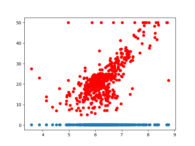
plt.scatter(X_rm, Y,color = 'red')
plt.scatter(X_rm,y_hat(k1, k2, b1, b2, X_rm))
plt.show()
# L2 loss function
def Loss(y_ture, y_hat):
return np.mean((np.array(y_ture) - np.array(y_hat)) ** 2)
# Partial derivative of b2
def partial_b2(y_ture, y_hat):
return -2 * np.mean(np.array(y_ture)-np.array(y_hat))
# Partial derivative of k2
def partial_k2(y_ture, y_hat, k1, b1, x):
s = 0
n = 0
for y_ture_i, y_hat_i, x_i in zip(y_ture, y_hat, x):
s += sigmoid(k1 * x_i + b1) * (y_ture_i - y_hat_i) * 2
n = n + 1
return -s/n
# Partial derivative of k1
def partial_k1(y_ture, y_hat, k1, b1, x):
s = 0
n = 0
for y_ture_i, y_hat_i, x_i in zip(y_ture, y_hat, x):
s += 2 * x_i * (y_ture_i - y_hat_i) * k2 * (sigmoid(k1 * x_i + b1) - sigmoid(k1 * x_i + b1) ** 2)
n = n + 1
return (-1.0 * s)/(1.0 * n)
# Partial derivative of b1
def partial_b1(y_ture, y_hat, k1, b1, x):
s = 0
n = 0
for y_ture_i, y_hat_i, x_i in zip(y_ture, y_hat, x):
s += 2 * (y_ture_i - y_hat_i) * k2 * (sigmoid(k1 * x_i + b1) - sigmoid(k1 * x_i + b1) ** 2)
n = n + 1
return (-1.0 * s)/(1.0 * n)
trying_time = 20000
min_loss = float('inf')
best_k1, best_b1 = None, None
best_k2, best_b2 = None, None
learning_rate = 1e-3
y_guess = y_hat(k1, k2, b1, b2, X_rm)
for i in range(trying_time):
# Compare the current loss to the minimum loss
y_guess = y_hat(k1, k2, b1, b2, X_rm)
loss = Loss(Y, y_guess)
if loss < min_loss:
best_k1 = k1
best_b1 = b1
best_k2 = k2
best_b2 = b2
min_loss = loss
if i % 1000 == 0:
print(min_loss)
# Find a more suitable k and b
k1 = k1 - partial_k1(Y, y_guess, k1, b1, X_rm) * learning_rate
b1 = b1 - partial_b1(Y, y_guess, k1, b1, X_rm) * learning_rate
k2 = k2 - partial_k2(Y, y_guess, k1, b1, X_rm) * learning_rate
b2 = b2 - partial_b2(Y, y_guess) * learning_rate
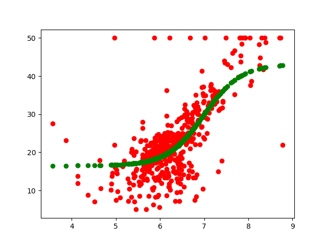
plt.scatter(X_rm, Y,color = 'red')
plt.scatter(X_rm, y_hat(best_k1, best_k2, best_b1, best_b2, X_rm), color='green')
print('The function represented is{} * sigmoid({} * x+ {} ) + {}'.format(best_k2,best_k1,best_b1,best_b2))
print('Loss is{}'.format(min_loss))
plt.show()
Training results: