introduction

The so-called sorting is the operation of arranging a string of records incrementally or decrementally according to the size of one or some keywords. Sorting algorithm is how to arrange records according to requirements. Sorting algorithm has received considerable attention in many fields, especially in the processing of large amounts of data. An excellent algorithm can save a lot of resources. Considering various limitations and specifications of data in various fields, it takes a lot of reasoning and analysis to get an excellent algorithm in line with the reality.

Two years ago, I was in Blog Garden Published an article Summary of the top ten classic sorting algorithms (including JAVA code implementation) The blog briefly introduces the ten classic sorting algorithms. However, in the previous blog, only the code implementation of the Java version is given, and there are some detailed errors. Therefore, I will write an article again today to deeply understand the principle and implementation of the next ten classic sorting algorithms.

brief introduction

Sorting algorithms can be divided into internal sorting and External sorting , the internal sort is to sort the data records in memory, while the external sort is to access the external memory during the sorting process because the sorted data is large and can not accommodate all the sorted records at one time. Common internal sorting algorithms include: insert sort, Hill sort, select sort, bubble sort, merge sort, quick sort, heap sort, cardinal sort, etc. This paper only explains the internal sorting algorithm. Summarize with a picture:

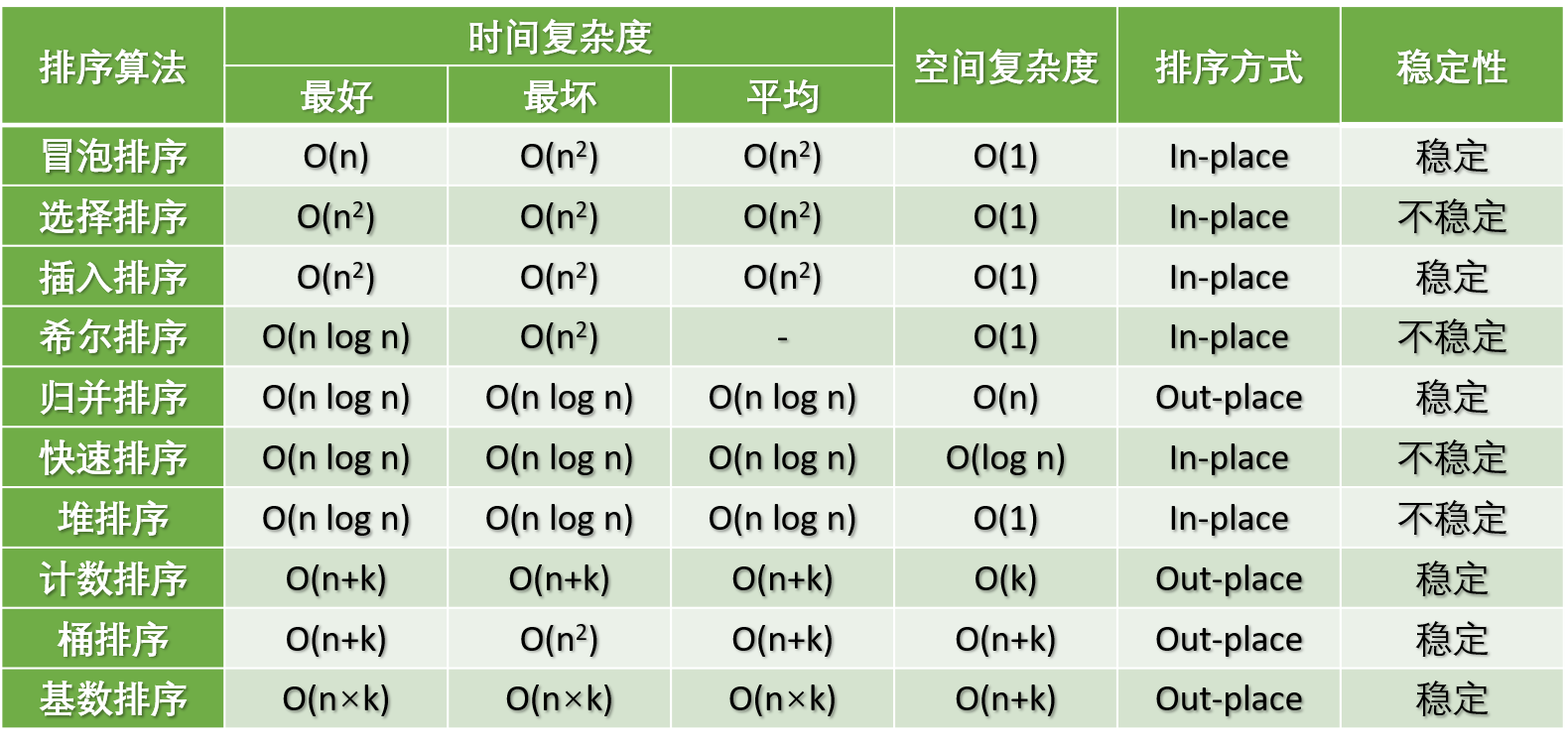
Explanation of picture terms:

• n: Data scale
• k: Number of "barrels"
• In place: it occupies constant memory and does not occupy additional memory
• Out place: use additional memory

Description of terms

• Stable: if A was in front of B and A=B, A will still be in front of B after sorting.
• Unstable: if A was originally in front of B and A=B, A may appear after B after sorting.
• Internal sorting: all sorting operations are completed in memory.
• External sorting: because the data is too large, the data is placed on the disk, and the sorting can only be carried out through the data transmission of disk and memory.
• Time complexity: it qualitatively describes the time spent in the execution of an algorithm.
• Spatial complexity: a qualitative description of the size of memory required for the execution of an algorithm.

Algorithm classification

Ten common sorting algorithms can be classified into two categories: comparative sorting and non comparative sorting.

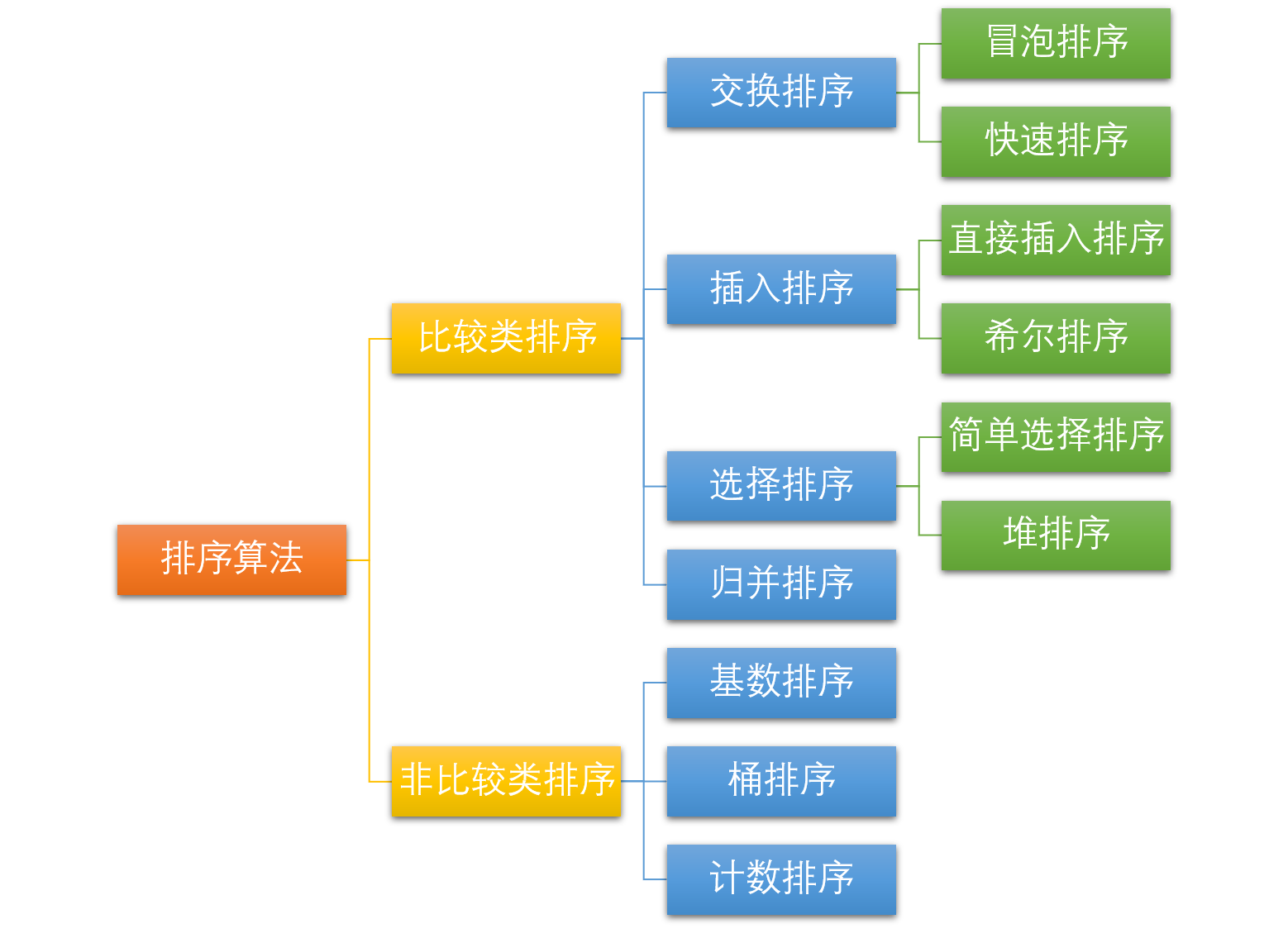
Common quick sort, merge sort, heap sort and bubble sort all belong to comparative sort algorithms. Comparison sort determines the relative order between elements through comparison. Because its time complexity can not exceed O(nlogn), it is also called nonlinear time comparison sort. In bubble sort, the problem scale is n, and because it needs to be compared n times, the average time complexity is O(n) ²). In sorting such as merge sort and quick sort, the problem scale is reduced to logn times by divide and conquer, so the time complexity is O(nlogn) on average.

The advantage of comparative sort is that it is suitable for data of all sizes and does not care about the distribution of data. It can be said that comparative sort is suitable for all situations that need to be sorted.

Count sort, cardinal sort and bucket sort belong to non comparison sort algorithms. Non comparison sort does not determine the relative order between elements through comparison, but determines how many elements should be sorted before each element. Because it can break through the lower bound of time based on comparison sort and run in linear time, it is called linear time non comparison sort The comparison sort only needs to determine the number of existing elements before each element, and all traversals can be solved. The time complexity of the algorithm is O(n).

The time complexity of non comparative sorting is low, but because non comparative sorting needs to occupy space to determine the unique location, it has certain requirements for data scale and data distribution.

Bubble sort

Bubble sorting is a simple sorting algorithm. It repeatedly traverses the sequence to be sorted, compares two elements in turn, and exchanges them if their order is wrong. The work of traversing the sequence is repeated until there is no need to exchange, which indicates that the sequence has been sorted. The name of this algorithm is because the smaller elements will be exchanged Slowly "float" to the top of the sequence.

Algorithm steps

1. Compare adjacent elements. If the first is larger than the second, swap them two;
2. Do the same for each pair of adjacent elements, from the first pair at the beginning to the last pair at the end, so that the last element should be the largest number;
3. Repeat the above steps for all elements except the last one;
4. Repeat steps 1 to 3 until the sorting is completed.

Graphic algorithm

code implementation

JAVA

/**
 * Bubble sorting
 * @param arr
 * @return arr
 */
public static int[] BubbleSort(int[] arr) {
    for (int i = 1; i < arr.length; i++) {
        // Set a flag, if true, that means the loop has not been swapped, 
        // that is, the sequence has been ordered, the sorting has been completed.
        boolean flag = true;
        for (int j = 0; j < arr.length - i; j++) {
            if (arr[j] > arr[j + 1]) {
                int tmp = arr[j];
                arr[j] = arr[j + 1];
                arr[j + 1] = tmp;
			    // Change flag
                flag = false;
            }
        }
        if (flag) {
            break;
        }
    }
    return arr;
}

Python

def BubbleSort(arr):
    for i in range(len(arr)):
        is_sorted = True
        for j in range(len(arr)-i-1):
            if arr[j] > arr[j+1]:
                arr[j], arr[j+1] = arr[j+1], arr[j]
                is_sorted = False
        if is_sorted:
            break
    return arr

Here, a small optimization is made for the code and the is_sorted Flag is added to optimize the optimal time complexity of the algorithm as O(n), that is, when the original input sequence is sorted, the time complexity of the algorithm is O(n).

Selection sort

Selective sorting is a simple and intuitive sorting algorithm. No matter what data goes in, it is O(n) ²) The smaller the data size, the better. The only advantage may be that it does not occupy additional memory space. Its working principle: first find the smallest (large) element in the unordered sequence, store it at the beginning of the sorted sequence, and then continue to find the smallest (large) element from the remaining unordered elements Element, and then put it at the end of the sorted sequence. And so on until all elements are sorted.

Algorithm steps

1. First, find the smallest (large) element in the unordered sequence and store it at the beginning of the sorted sequence
2. Then continue to find the smallest (large) element from the remaining unordered elements, and then put it at the end of the sorted sequence.
3. Repeat step 2 until all elements are sorted.

Graphic algorithm

code implementation

JAVA

/**
 * Select sort
 * @param arr
 * @return arr
 */
public static int[] SelectionSort(int[] arr) {
    for (int i = 0; i < arr.length - 1; i++) {
        int minIndex = i;
        for (int j = i + 1; j < arr.length; j++) {
            if (arr[j] < arr[minIndex]) {
                minIndex = j;
            }
        }
        if (minIndex != i) {
            int tmp = arr[i];
            arr[i] = arr[minIndex];
            arr[minIndex] = tmp;
        }
    }
    return arr;
}

Python

def SelectionSort(arr):
    for i in range(len(arr)-1):
        # Record the index of the minimum value
        minIndex = i
        for j in range(i+1, len(arr)):
            if arr[j] < arr[minIndex]:
                minIndex = j
        if minIndex != i:
            arr[i], arr[minIndex] = arr[minIndex], arr[i]
    return arr

Insertion sort

Insertion sort is a simple and intuitive sorting algorithm. Its working principle is to construct an ordered sequence. For unordered data, scan back and forward in the sorted sequence to find the corresponding position and insert. Insertion sort is usually implemented by in place sort (i.e. sort that only needs O(1) extra space) Therefore, in the process of scanning from back to front, it is necessary to repeatedly move the sorted elements back step by step to provide insertion space for the latest elements.

Although the code implementation of insertion sorting is not as simple and rough as bubble sorting and selection sorting, its principle should be the easiest to understand, because anyone who has played poker should be able to understand it. Insert sort is the simplest and most intuitive sort algorithm. Its working principle is to build an ordered sequence. For unordered data, scan back and forward in the sorted sequence to find the corresponding position and insert.

Like bubble sort, insertion sort also has an optimization algorithm called split half insertion.

Algorithm steps

1. Starting from the first element, the element can be considered to have been sorted;
2. Take out the next element and scan from back to front in the sorted element sequence;
3. If the element (sorted) is larger than the new element, move the element to the next position;
4. Repeat step 3 until the sorted element is found to be less than or equal to the position of the new element;
5. After inserting the new element into this position;
6. Repeat steps 2 to 5.

Graphic algorithm

code implementation

JAVA

/**
 * Insert sort
 * @param arr
 * @return arr
 */
public static int[] InsertionSort(int[] arr) {
    for (int i = 1; i < arr.length; i++) {
        int preIndex = i - 1;
        int current = arr[i];
        while (preIndex >= 0 && current < arr[preIndex]) {
            arr[preIndex + 1] = arr[preIndex];
            preIndex -= 1;
        }
        arr[preIndex + 1] = current;
    }
    return arr;
}

Python

def InsertionSort(arr):
    for i in range(1, len(arr)):
        preIndex = i-1
        current = arr[i]
        while preIndex >= 0 and current < arr[preIndex]:
            arr[preIndex+1] = arr[preIndex]
            preIndex -= 1
        arr[preIndex+1] = current
    return arr

Shell sort

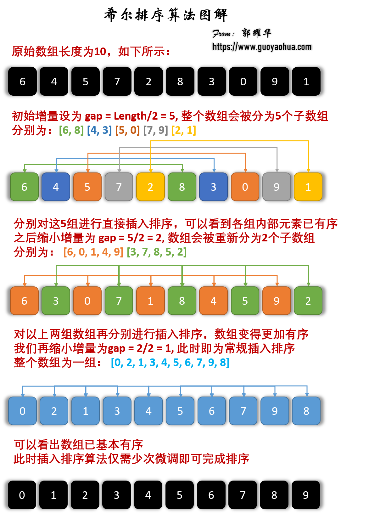
Hill sorting is a sort algorithm proposed by Donald shell in 1959. Hill sort is also an insertion sort. It is a more efficient version of simple insertion sort after improvement, also known as decreasing incremental sort algorithm. At the same time, the algorithm breaks through O(n) ²) One of the first algorithms.

The basic idea of Hill sort is to divide the whole record sequence to be sorted into several subsequences for direct insertion sort. When the records in the whole sequence are "basically orderly", all records will be directly inserted and sorted in turn.

Algorithm steps

Let's look at the basic steps of hill sorting. Here, we select the increment gap=length/2, reduce the increment and continue to use gap = gap/2. This incremental selection can be expressed in a sequence, {n / 2, (n / 2) / 2,..., 1} , called the incremental sequence. The selection and proof of the incremental sequence sorted by hill is a mathematical problem. The incremental sequence we selected is commonly used and is also the increment suggested by hill, called Hill increment, but in fact, this incremental sequence is not optimal. Here we use hill increment as an example.

First, divide the whole record sequence to be sorted into several subsequences for direct insertion sorting. The specific algorithm description is as follows:

• Select an incremental sequence {t1, t2,..., tk}, where (Ti > TJ, I < J, tk = 1);
• Sort the sequence k times according to the number of incremental sequences k;
• For each sorting, the sequence to be sorted is divided into several subsequences with length m according to the corresponding increment t, and each sub table is directly inserted and sorted. Only when the increment factor is 1, the whole sequence is treated as a table, and the table length is the length of the whole sequence.

Graphic algorithm

code implementation

JAVA

/**
 * Shell Sort 
 *
 * @param arr
 * @return arr
 */
public static int[] ShellSort(int[] arr) {
    int n = arr.length;
    int gap = n / 2;
    while (gap > 0) {
        for (int i = gap; i < n; i++) {
            int current = arr[i];
            int preIndex = i - gap;
            // Insertion sort
            while (preIndex >= 0 && arr[preIndex] > current) {
                arr[preIndex + gap] = arr[preIndex];
                preIndex -= gap;
            }
            arr[preIndex + gap] = current;

        }
        gap /= 2;
    }
    return arr;
}

Python

def ShellSort(arr):
    n = len(arr)
    # Initial step size
    gap = n // 2
    while gap > 0:
        for i in range(gap, n):
            # Insert sort by step
            current = arr[i]
            preIndex = i - gap
            # Insert sort
            while preIndex >= 0 and arr[preIndex] > current:
                arr[preIndex+gap] = arr[preIndex]
                preIndex -= gap
            arr[preIndex+gap] = current
        # Get new step size
        gap = gap // 2
    return arr

Merge sort

Merge sort is an effective sort algorithm based on merge operation. The algorithm adopts divide and conquer Merge sort is a stable sort method. Merge the ordered subsequences to obtain a completely ordered sequence; that is, order each subsequence first, and then order the subsequence segments. If two ordered tables are merged into one ordered table, it is called 2-way merge.

Like the selective sort, the performance of merge sort is not affected by the input data, but it performs much better than the selective sort, because it is always O(nlogn) time complexity. The cost is the need for additional memory space.

Algorithm steps

The merge sort algorithm is a recursive process. The boundary condition is that when the input sequence has only one element, it will return directly. The specific process is as follows:

1. If there is only one element in the input, it will be returned directly. Otherwise, the input sequence with length n will be divided into two subsequences with length n/2;
2. Merge and sort the two subsequences respectively to make the subsequences into an ordered state;
3. Set two pointers to the starting positions of two sorted subsequences respectively;
4. Compare the elements pointed to by the two pointers, select the relatively small elements and put them into the merge space (used to store the sorting results), and move the pointer to the next position;
5. Repeat steps 3 to 4 until a pointer reaches the end of the sequence;
6. Copy all the remaining elements of another sequence directly to the end of the merged sequence.

Graphic algorithm

code implementation

JAVA

/**
 * Merge sort
 *
 * @param arr
 * @return arr
 */
public static int[] MergeSort(int[] arr) {
    if (arr.length <= 1) {
        return arr;
    }
    int middle = arr.length / 2;
    int[] arr_1 = Arrays.copyOfRange(arr, 0, middle);
    int[] arr_2 = Arrays.copyOfRange(arr, middle, arr.length);
    return Merge(MergeSort(arr_1), MergeSort(arr_2));
}

/**
 * Merge two sorted arrays
 * 
 * @param arr_1
 * @param arr_2
 * @return sorted_arr
 */
public static int[] Merge(int[] arr_1, int[] arr_2) {
    int[] sorted_arr = new int[arr_1.length + arr_2.length];
    int idx = 0, idx_1 = 0, idx_2 = 0;
    while (idx_1 < arr_1.length && idx_2 < arr_2.length) {
        if (arr_1[idx_1] < arr_2[idx_2]) {
            sorted_arr[idx] = arr_1[idx_1];
            idx_1 += 1;
        } else {
            sorted_arr[idx] = arr_2[idx_2];
            idx_2 += 1;
        }
        idx += 1;
    }
    if (idx_1 < arr_1.length) {
        while (idx_1 < arr_1.length) {
            sorted_arr[idx] = arr_1[idx_1];
            idx_1 += 1;
            idx += 1;
        }
    } else {
        while (idx_2 < arr_2.length) {
            sorted_arr[idx] = arr_2[idx_2];
            idx_2 += 1;
            idx += 1;
        }
    }
    return sorted_arr;
}

Python

def Merge(arr_1, arr_2):
    sorted_arr = []
    idx_1 = 0
    idx_2 = 0
    while idx_1 < len(arr_1) and idx_2 < len(arr_2):
        if arr_1[idx_1] < arr_2[idx_2]:
            sorted_arr.append(arr_1[idx_1])
            idx_1 += 1
        else:
            sorted_arr.append(arr_2[idx_2])
            idx_2 += 1
    if idx_1 < len(arr_1):
        while idx_1 < len(arr_1):
            sorted_arr.append(arr_1[idx_1])
            idx_1 += 1
    else:
        while idx_2 < len(arr_2):
            sorted_arr.append(arr_2[idx_2])
            idx_2 += 1
    return sorted_arr

def MergeSort(arr):
    if len(arr) <= 1:
        return arr
    mid = int(len(arr)/2)
    arr_1, arr_2 = arr[:mid], arr[mid:]
    return Merge(MergeSort(arr_1), MergeSort(arr_2))

algorithm analysis

Stability: stable

Time complexity: best: O(nlogn) worst: O(nlogn) average: O(nlogn)

Space complexity: O(n)

Quick sort

Quick sort uses the idea of divide and conquer, as well as merge sort. At first glance, quick sort and merge sort are very similar. They both reduce the problem, sort the substring first, and then merge. The difference is that quick sort takes one more step when dividing the sub problem, and divides the divided two groups of data into one large and one small, so that it does not have to be like merge in the final merge But because of this, the uncertainty of division makes the time complexity of quick sorting unstable.

Basic idea of quick sorting: the sequence to be arranged is divided into two independent parts by one-time sorting. If the elements recorded in one part are smaller than those in the other part, the two molecular sequences can be sorted separately to achieve the order of the whole sequence.

Algorithm steps

Quick sort use Divide and conquer (Divide and conquer) strategy to divide a sequence into two smaller and larger subsequences, and then sort the two subsequences recursively. The specific algorithm is described as follows:

1. Randomly pick out an element from the sequence as a "pivot";
2. Rearrange the sequence. Put all elements smaller than the benchmark value in front of the benchmark, and all elements larger than the benchmark value behind the benchmark (the same number can be on either side). After this operation, the benchmark is in the middle of the sequence. This is called partition operation;
3. Recursively sort subsequences smaller than the reference value element and subsequences larger than the reference value element.

Graphic algorithm

code implementation

JAVA

/**
 * Swap the two elements of an array
 * @param array
 * @param i
 * @param j
 */
private static void swap(int[] arr, int i, int j) {
    int tmp = arr[i];
    arr[i] = arr[j];
    arr[j] = tmp;
}

/**
 * Partition function
 * @param arr
 * @param left
 * @param right
 * @return small_idx
 */
private static int Partition(int[] arr, int left, int right) {
    if (left == right) {
        return left;
    }
    // random pivot
    int pivot = (int) (left + Math.random() * (right - left + 1));
    swap(arr, pivot, right);
    int small_idx = left;
    for (int i = small_idx; i < right; i++) {
        if (arr[i] < arr[right]) {
            swap(arr, i, small_idx);
            small_idx++;
        }
    }
    swap(arr, small_idx, right);
    return small_idx;
}

/**
 * Quick sort function
 * @param arr
 * @param left
 * @param right
 * @return arr
 */
public static int[] QuickSort(int[] arr, int left, int right) {
    if (left < right) {
        int pivotIndex = Partition(arr, left, right);
        sort(arr, left, pivotIndex - 1);
        sort(arr, pivotIndex + 1, right);
    }
    return arr;
}

Python

def QuickSort(arr, left=None, right=None):
    left = 0 if left == None else left
    right = len(arr)-1 if right == None else right
    if left < right:
        pivotIndex = Partition(arr, left, right)
        QuickSort(arr, left, pivotIndex-1)
        QuickSort(arr, pivotIndex+1, right)
    return arr

def Partition(arr, left, right):
    if left == right:
        return left
    # Random pivot
    swap(arr, random.randint(left, right), right)
    pivot = right
    small_idx = left
    for i in range(small_idx, pivot):
        if arr[i] < arr[pivot]:
            swap(arr, i, small_idx)
            small_idx += 1
    swap(arr, small_idx, pivot)
    return small_idx

def swap(arr, i, j):
    arr[i], arr[j] = arr[j], arr[i]

algorithm analysis

Stability: unstable

Time complexity: best: O(nlogn) worst: O(nlogn) average: O(nlogn)

Spatial complexity: O(nlogn)

Heap sort

Heap sorting is a sort algorithm designed by using heap as a data structure. Heap is a structure similar to a complete binary tree and satisfies the nature of heap: that is, the value of child node is always less than (or greater than) its parent node.

Algorithm steps

1. The initial waiting sequence (R1, R2,..., Rn) is constructed into a large top heap, which is the initial disordered region;
2. Exchange the top element R[1] with the last element R[n], and a new disordered region (R1, R2,..., Rn-1) and a new ordered region (Rn) are obtained, and R[1, 2,..., n-1] < = R[n];
3. Since the new heap top R[1] may violate the nature of the heap after exchange, it is necessary to adjust the current unordered area (R1, R2,..., Rn-1) to a new heap, and then exchange R[1] with the last element of the unordered area again to obtain a new unordered area (R1, R2,..., Rn-2) and a new ordered area (RN-1, Rn-1). Repeat this process until the number of elements in the ordered area is n-1, and the whole sorting process is completed.

Graphic algorithm

code implementation

JAVA

// Global variable that records the length of an array;
static int heapLen;

/**
 * Swap the two elements of an array
 * @param arr
 * @param i
 * @param j
 */
private static void swap(int[] arr, int i, int j) {
    int tmp = arr[i];
    arr[i] = arr[j];
    arr[j] = tmp;
}

/**
 * Build Max Heap
 * @param arr
 */
private static void buildMaxHeap(int[] arr) {
    for (int i = arr.length / 2 - 1; i >= 0; i--) {
        heapify(arr, i);
    }
}

/**
 * Adjust it to the maximum heap
 * @param arr
 * @param i
 */
private static void heapify(int[] arr, int i) {
    int left = 2 * i + 1;
    int right = 2 * i + 2;
    int largest = i;
    if (right < heapLen && arr[right] > arr[largest]) {
        largest = right;
    }
    if (left < heapLen && arr[left] > arr[largest]) {
        largest = left;
    }
    if (largest != i) {
        swap(arr, largest, i);
        heapify(arr, largest);
    }
}

/**
 * Heap Sort
 * @param arr
 * @return
 */
public static int[] HeapSort(int[] arr) {
    // index at the end of the heap
    heapLen = arr.length;
    // build MaxHeap
    buildMaxHeap(arr);
    for (int i = arr.length - 1; i > 0; i--) {
        // Move the top of the heap to the tail of the heap in turn
        swap(arr, 0, i);
        heapLen -= 1;
        heapify(arr, 0);
    }
    return arr;
}

Python

def HeapSort(arr):
    global heapLen
    # Index used to mark the end of the heap
    heapLen = len(arr)
    # Build maximum heap
    buildMaxHeap(arr)
    for i in range(len(arr)-1, 0, -1):
        # Move the top of the heap to the end of the heap in turn
        swap(arr, 0, i)
        heapLen -= 1
        heapify(arr, 0)
    return arr

def buildMaxHeap(arr):
    for i in range(len(arr)//2-1, -1, -1):
        heapify(arr, i)

def heapify(arr, i):
    left = 2*i + 1
    right = 2*i + 2
    largest = i
    if right < heapLen and arr[right] > arr[largest]:
        largest = right
    if left < heapLen and arr[left] > arr[largest]:
        largest = left
    if largest != i:
        swap(arr, largest, i)
        heapify(arr, largest)

def swap(arr, i, j):
    arr[i], arr[j] = arr[j], arr[i]

algorithm analysis

Stability: unstable

Time complexity: best: O(nlogn) worst: O(nlogn) average: O(nlogn)

Space complexity: O(1)

Counting sort

The core of counting sorting is to convert the input data values into keys and store them in the additional array space. As a sort with linear time complexity, count sort requires that the input data must be integers with a certain range.

Counting sort is A stable sorting algorithm. Count sorting uses an additional array C, where the ith element is the number of elements with A value equal to i in the array A to be sorted. Then arrange the elements in A in the correct position according to array C. It can only sort integers.

Algorithm steps

1. Find out the maximum value max and minimum value min in the array;
2. Create a new array C, whose length is max min + 1, and the default values of its elements are 0;
3. Traverse the element A[i] in the original array A, take A[i]-min as the index of the C array, and take the occurrence times of the element in A as the value of C[A[i]-min];
4. For C array deformation, the value of the new element is the sum of the element and the value of the previous element, that is, when I > 1, C[i] = C[i] + C[i-1];
5. Create the result array R with the same length as the original array.
6. Traverse the element A[i] in the original array A from back to front, use A[i] minus the minimum value min as the index, and find the corresponding value C[A[i]-min] in the count array C. C[A[i]-min]-1 is the position of A[i] in the result array R. after these operations, reduce count[A[i]-min] by 1.

Graphic algorithm

code implementation

JAVA

/**
 * Gets the maximum and minimum values in the array
 * 
 * @param arr
 * @return
 */
private static int[] getMinAndMax(int[] arr) {
    int maxValue = arr[0];
    int minValue = arr[0];
    for (int i = 0; i < arr.length; i++) {
        if (arr[i] > maxValue) {
            maxValue = arr[i];
        } else if (arr[i] < minValue) {
            minValue = arr[i];
        }
    }
    return new int[] { minValue, maxValue };
}

/**
 * Counting Sort
 * 
 * @param arr
 * @return
 */
public static int[] CountingSort(int[] arr) {
    if (arr.length < 2) {
        return arr;
    }
    int[] extremum = getMinAndMax(arr);
    int minValue = extremum[0];
    int maxValue = extremum[1];
    int[] countArr = new int[maxValue - minValue + 1];
    int[] result = new int[arr.length];

    for (int i = 0; i < arr.length; i++) {
        countArr[arr[i] - minValue] += 1;
    }
    for (int i = 1; i < countArr.length; i++) {
        countArr[i] += countArr[i - 1];
    }
    for (int i = arr.length - 1; i >= 0; i--) {
        int idx = countArr[arr[i] - minValue] - 1;
        result[idx] = arr[i];
        countArr[arr[i] - minValue] -= 1;
    }
    return result;
}

Python

def CountingSort(arr):
    if arr.size < 2:
        return arr
    minValue, maxValue = getMinAndMax(arr)
    countArr = [0]*(maxValue-minValue+1)
    resultArr = [0]*len(arr)
    for i in range(len(arr)):
        countArr[arr[i]-minValue] += 1
    for i in range(1, len(countArr)):
        countArr[i] += countArr[i-1]
    for i in range(len(arr)-1, -1, -1):
        idx = countArr[arr[i]-minValue]-1
        resultArr[idx] = arr[i]
        countArr[arr[i]-minValue] -= 1
    return resultArr


def getMinAndMax(arr):
    maxValue = arr[0]
    minValue = arr[0]
    for i in range(len(arr)):
        if arr[i] > maxValue:
            maxValue = arr[i]
        elif arr[i] < minValue:
            minValue = arr[i]
    return minValue, maxValue

algorithm analysis

When the input element is n integers between 0 and K, its running time is O(n+k). Counting sort is not a comparison sort, and the sorting speed is faster than any comparison sort algorithm. Since the length of array C used for counting depends on the range of data in the array to be sorted (equal to the difference between the maximum and minimum values of the array to be sorted plus 1), counting sorting requires a lot of additional memory space for arrays with large data range.

Stability: stable

Time complexity: best: O(n+k) worst: O(n+k) average: O(n+k)

Space complexity: O(k)

Bucket sort

Bucket sorting is an upgraded version of counting sorting. It makes use of the mapping relationship of the function. The key to efficiency lies in the determination of the mapping function. In order to make bucket sorting more efficient, we need to do these two things:

1. Increase the number of barrels as much as possible with sufficient additional space
2. The mapping function used can evenly distribute the input N data into K buckets

Working principle of bucket sorting: assuming that the input data is uniformly distributed, divide the data into a limited number of buckets, and sort each bucket separately (it is possible to use other sorting algorithms or continue to use bucket sorting recursively).

Algorithm steps

1. Set a bucket size as how many different values can be placed in each bucket;
2. Traverse the input data and map the data to the corresponding bucket in turn;
3. To sort each non empty bucket, you can use other sorting methods or recursive bucket sorting;
4. Concatenate ordered data from non empty buckets.

Graphic algorithm

code implementation

JAVA

/**
 * Gets the maximum and minimum values in the array
 * @param arr
 * @return
 */
private static int[] getMinAndMax(List<Integer> arr) {
    int maxValue = arr.get(0);
    int minValue = arr.get(0);
    for (int i : arr) {
        if (i > maxValue) {
            maxValue = i;
        } else if (i < minValue) {
            minValue = i;
        }
    }
    return new int[] { minValue, maxValue };
}

/**
 * Bucket Sort
 * @param arr
 * @return
 */
public static List<Integer> BucketSort(List<Integer> arr, int bucket_size) {
    if (arr.size() < 2 || bucket_size == 0) {
        return arr;
    }
    int[] extremum = getMinAndMax(arr);
    int minValue = extremum[0];
    int maxValue = extremum[1];
    int bucket_cnt = (maxValue - minValue) / bucket_size + 1;
    List<List<Integer>> buckets = new ArrayList<>();
    for (int i = 0; i < bucket_cnt; i++) {
        buckets.add(new ArrayList<Integer>());
    }
    for (int element : arr) {
        int idx = (element - minValue) / bucket_size;
        buckets.get(idx).add(element);
    }
    for (int i = 0; i < buckets.size(); i++) {
        if (buckets.get(i).size() > 1) {
            buckets.set(i, sort(buckets.get(i), bucket_size / 2));
        }
    }
    ArrayList<Integer> result = new ArrayList<>();
    for (List<Integer> bucket : buckets) {
        for (int element : bucket) {
            result.add(element);
        }
    }
    return result;
}

Python

def BucketSort(arr, bucket_size):
    if len(arr) < 2 or bucket_size == 0:
        return arr
    minValue, maxValue = getMinAndMax(arr)
    bucket_cnt = (maxValue-minValue)//bucket_size+1
    bucket = [[] for i in range(bucket_cnt)]
    for i in range(len(arr)):
        idx = (arr[i]-minValue) // bucket_size
        bucket[idx].append(arr[i])
    for i in range(len(bucket)):
        if len(bucket[i]) > 1:
            # Bucket sorting is used recursively, and other sorting algorithms can also be used
            bucket[i] = BucketSort(bucket[i], bucket_size//2)
    result = []
    for i in range(len(bucket)):
        for j in range(len(bucket[i])):
            result.append(bucket[i][j])
    return result


def getMinAndMax(arr):
    maxValue = arr[0]
    minValue = arr[0]
    for i in range(len(arr)):
        if arr[i] > maxValue:
            maxValue = arr[i]
        elif arr[i] < minValue:
            minValue = arr[i]
    return minValue, maxValue

algorithm analysis

Stability: stable

Time complexity: best: O(n+k) worst: O(n ²) Average: O(n+k)

Space complexity: O(k)

Radix sort

Cardinality sorting is also a non comparison sorting algorithm. It sorts each digit in the element, starting from the lowest bit, with a complexity of O(n) × k) , n is the length of the array, and K is the maximum number of bits of elements in the array;

Cardinality sorting is to sort first according to the low order and then collect; then sort according to the high order and then collect; and so on until the highest order. Sometimes some attributes have priority order, sort according to the low priority first, and then sort according to the high priority. The last order is the high priority first, and the low priority with the same high priority first. Cardinality sorting is based on score Do not sort, collect separately, so it is stable.

Algorithm steps

1. Obtain the maximum number in the array and the number of bits, that is, the number of iterations N (for example, if the maximum value in the array is 1000, then N=4);
2. A is the original array, and each bit is taken from the lowest bit to form a radius array;
3. Count and sort the radix (using the characteristics that count sorting is suitable for a small range of numbers);
4. Assign radix to the original array in turn;
5. Repeat steps 2 ~ 4 N times

Graphic algorithm

code implementation

JAVA

/**
 * Radix Sort
 * 
 * @param arr
 * @return
 */
public static int[] RadixSort(int[] arr) {
    if (arr.length < 2) {
        return arr;
    }
    int N = 1;
    int maxValue = arr[0];
    for (int element : arr) {
        if (element > maxValue) {
            maxValue = element;
        }
    }
    while (maxValue / 10 != 0) {
        maxValue = maxValue / 10;
        N += 1;
    }
    for (int i = 0; i < N; i++) {
        List<List<Integer>> radix = new ArrayList<>();
        for (int k = 0; k < 10; k++) {
            radix.add(new ArrayList<Integer>());
        }
        for (int element : arr) {
            int idx = (element / (int) Math.pow(10, i)) % 10;
            radix.get(idx).add(element);
        }
        int idx = 0;
        for (List<Integer> l : radix) {
            for (int n : l) {
                arr[idx++] = n;
            }
        }
    }
    return arr;
}

Python

def RadixSort(arr):
    if len(arr) < 2:
        return arr
    maxValue = arr[0]
    N = 1
    for i in range(len(arr)):
        if arr[i] > maxValue:
            maxValue = arr[i]
    while maxValue // 10 != 0:
        maxValue = maxValue//10
        N += 1
    for n in range(N):
        radix = [[] for i in range(10)]
        for i in range(len(arr)):
            idx = arr[i]//(10**n) % 10
            radix[idx].append(arr[i])
        idx = 0
        for j in range(len(radix)):
            for k in range(len(radix[j])):
                arr[idx] = radix[j][k]
                idx += 1
    return arr

algorithm analysis

Stability: stable

Time complexity: optimal: O(n) × k) Worst: O(n) × k) Average: O(n) × k)

Spatial complexity: O(n+k)

Cardinality sort vs count sort vs bucket sort

These three sorting algorithms all use the concept of bucket, but there are obvious differences in the use of bucket:

• Cardinality sorting: allocate buckets according to each number of key value
• Count sorting: each bucket stores only one key value
• Bucket sorting: each bucket stores a certain range of values

Reference articles

https://www.cnblogs.com/guoyaohua/p/8600214.html

https://en.wikipedia.org/wiki/Sorting_algorithm

https://sort.hust.cc/