Introduction to deep learning series 20: LSTM recurrent neural network to solve the problem of international air passenger prediction

Hello, my technician Howzit, this is the 20th part of the introduction series of in-depth learning. Welcome to communicate with us!

Time series prediction is a difficult problem in prediction modeling. Unlike regression prediction, time series also increases the complexity of dependence in the sequence in the input variables. There is a powerful neural network dedicated to dealing with timing dependence problems, which we call recursive neural network * * (RNN). LSTM is a kind of recurrent neural network. It can be successfully applied in deep learning, mainly because its structure can be successfully trained. In this lesson, you will learn how to develop LSTM network through Keras deep learning library to solve the problem of time series prediction. After completing this lesson, you will learn how to implement and develop LSTM * * network to solve your own timing problems and other timing problems.

You will understand:

How to develop LSTM network and transform time series prediction problem into regression problem.
Aiming at the timing problem, we use window and time step to develop LSTM network.
In a very long sequence, how to use the LSTM network with saved state for development and prediction.

For the standard time series prediction problem, we will develop multiple LSTM neural units. The following questions and the selected configuration are for illustration and are not optimal. The following example formally introduces how to develop its own LSTM neural network and solve the problem of time series prediction.

Let's start.

1 LSTM network for regression

The problem of International Air Passenger Forecasting in the last section will be reconsidered in this class. We can translate the problem into a regression problem, just as we did in the last class. In other words, given the number of passengers in this month, the number of passengers in the next month (in 1000) is obtained. This example will reuse the data loading and data preprocessing of the previous lesson. Especially create_data() function.

LSTMs neural network is sensitive to data size, especially using sigmoid (default) and tanh activation function. Regularizing data between 0-1 is called regularization. We can regularize the data through MinMaxScaler preprocessing from the scikit learn library.

# normalize the dataset 
scaler = MinMaxScaler(feature_range=(0, 1)) 
dataset = scaler.fit_transform(dataset)

The expected input data * * (X) * * of the LSTM network is a specified format: [samples,time steps,features]. The data form we preprocess is: [samples,features]. For each sample, we define the problem as a time step. Using numpy.reshape(), we can convert our preprocessed training set and test set into our desired structure:

# reshape input to be [samples, time steps, features] 
trainX = numpy.reshape(trainX, (trainX.shape[0], 1, trainX.shape[1])) 
testX = numpy.reshape(testX, (testX.shape[0], 1, testX.shape[1]))

We are now ready to design and fit our LSTM network for the whole problem. The network has an input layer of an input neuron, a hidden layer with four LSTM units, and an output layer for predicting an output value. The default activation function sigmoid is used in the LSTM memory unit. The network is trained 100 times and the batch size is 1.

# create and fit the LSTM network 
model = Sequential() 
model.add(LSTM(4, input_shape=(1, look_back)))
model.add(Dense(1)) 
model.compile(loss='mean_squared_error', optimizer='adam') 
model.fit(trainX, trainY, epochs=100, batch_size=1, verbose=2)

For completeness, here is the whole code.

# LSTM for international airline passengers problem with regression framing  
import math  
  
import matplotlib.pyplot as plt  
import numpy  
from keras.layers import Dense  
from keras.layers import LSTM  
from keras.models import Sequential  
from pandas import read_csv  
from sklearn.metrics import mean_squared_error  
from sklearn.preprocessing import MinMaxScaler  
  
  
# convert an array of values into a dataset matrix  
def create_dataset(dataset, look_back=1):  
    dataX, dataY = [], []  
    for i in range(len(dataset) - look_back - 1):  
        a = dataset[i:(i + look_back), 0]  
        dataX.append(a)  
        dataY.append(dataset[i + look_back, 0])  
    return numpy.array(dataX), numpy.array(dataY)  
  
  
# fix random seed for reproducibility  
numpy.random.seed(7)  

# load the dataset  
dataframe = read_csv('international-airline-passengers.csv', usecols=[1], engine='python',  
                     skipfooter=3)  
dataset = dataframe.values  
dataset = dataset.astype('float32')  

# normalize the dataset  
scaler = MinMaxScaler(feature_range=(0, 1))  
dataset = scaler.fit_transform(dataset)  

# split into train and test sets  
train_size = int(len(dataset) * 0.67)  
test_size = len(dataset) - train_size  
train, test = dataset[0:train_size, :], dataset[train_size:len(dataset), :]  

# reshape into X=t and Y=t+1  
look_back = 1  
trainX, trainY = create_dataset(train, look_back)  
testX, testY = create_dataset(test, look_back)  

# reshape input to be [samples, time steps, features]  
trainX = numpy.reshape(trainX, (trainX.shape[0], 1, trainX.shape[1]))  
testX = numpy.reshape(testX, (testX.shape[0], 1, testX.shape[1]))  

# create and fit the LSTM network  
model = Sequential()  
model.add(LSTM(4, input_shape=(1, look_back)))  
model.add(Dense(1))  
model.compile(loss='mean_squared_error', optimizer='adam')  
model.fit(trainX, trainY, epochs=100, batch_size=1, verbose=2)  

# make predictions  
trainPredict = model.predict(trainX)  
testPredict = model.predict(testX)  

# invert predictions  
trainPredict = scaler.inverse_transform(trainPredict)  
trainY = scaler.inverse_transform([trainY])  
testPredict = scaler.inverse_transform(testPredict)  
testY = scaler.inverse_transform([testY])  

# calculate root mean squared error  
trainScore = math.sqrt(mean_squared_error(trainY[0], trainPredict[:, 0]))  
print('Train Score: %.2f RMSE' % (trainScore))  
testScore = math.sqrt(mean_squared_error(testY[0], testPredict[:, 0]))  
print('Test Score: %.2f RMSE' % (testScore))  

# shift train predictions for plotting  
trainPredictPlot = numpy.empty_like(dataset)  
trainPredictPlot[:, :] = numpy.nan  
trainPredictPlot[look_back:len(trainPredict) + look_back, :] = trainPredict  

# shift test predictions for plotting  
testPredictPlot = numpy.empty_like(dataset)  
testPredictPlot[:, :] = numpy.nan  
testPredictPlot[len(trainPredict) + (look_back * 2) + 1:len(dataset) - 1, :] = testPredict  

# plot baseline and predictions  
plt.plot(scaler.inverse_transform(dataset))  
plt.plot(trainPredictPlot)  
plt.plot(testPredictPlot)  
plt.show()

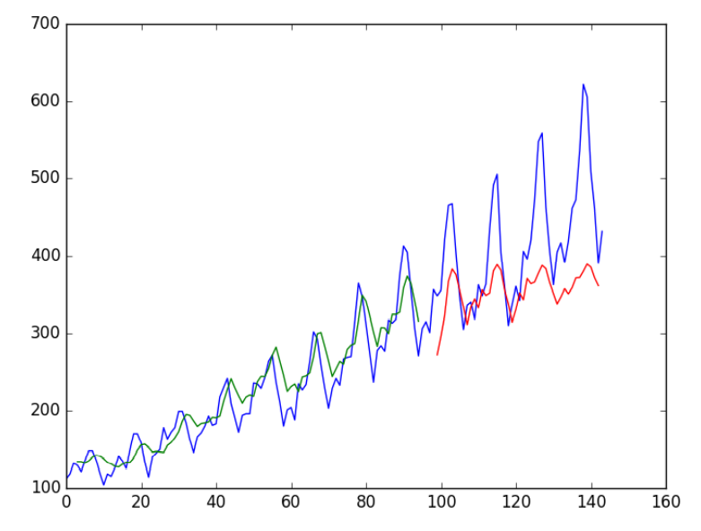
Run this model and get the following results:

Epoch 96/100
 - 0s - loss: 0.0020
Epoch 97/100
 - 0s - loss: 0.0019
Epoch 98/100
 - 0s - loss: 0.0019
Epoch 99/100
 - 0s - loss: 0.0019
Epoch 100/100
 - 0s - loss: 0.0019
Train Score: 22.34 RMSE
Test Score: 45.89 RMSE

We can see that the fitting results of the model on the training set and the test set are good.

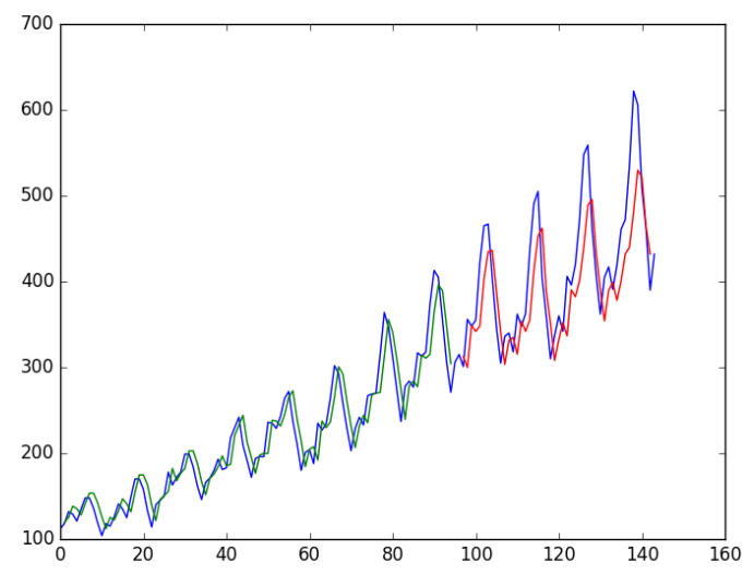
We can see that the model obtains 23 passenger errors (unit 1000) in the training set and 52 errors in the test set.

2 LSTM regression using Window method

We can also restate this problem so that multiple time steps can predict the next time, which is called window, and its size is set according to the problem. For example, given the current time * * (T) * *, we want to predict the value of the next time * * (t+1) * * in the sequence. We can use the current time (T) and the first two times (t-1 and t-2) as input variables. When the problem is described as a regression problem, its input variables are t-2, T-1, t and output variables are t+1.

Create created in the previous lesson_ The dataset () function allows us to set look_ The back parameter is increased from 1 to 3 to create the timing problem format. The sample format of the dataset is as follows:

X1   X2  X3  Y 
112 118 132 129 
118 132 129 121 
132 129 121 135 
129 121 135 148 
121 135 148 148

We rerun the example of large window in the previous lesson. For completeness, we put the whole code of large window below:

# LSTM for international airline passengers problem with window regression framing  

import math  
  
import matplotlib.pyplot as plt  
import numpy  
from keras.layers import Dense  
from keras.layers import LSTM  
from keras.models import Sequential  
from pandas import read_csv  
from sklearn.metrics import mean_squared_error  
from sklearn.preprocessing import MinMaxScaler  
  
  
# convert an array of values into a dataset matrix  
def create_dataset(dataset, look_back=1):  
    dataX, dataY = [], []  
    for i in range(len(dataset) - look_back - 1):  
        a = dataset[i:(i + look_back), 0]  
        dataX.append(a)  
        dataY.append(dataset[i + look_back, 0])  
    return numpy.array(dataX), numpy.array(dataY)  
  
  
# fix random seed for reproducibility  
numpy.random.seed(7)  
# load the dataset  
dataframe = read_csv('international-airline-passengers.csv', usecols=[1], engine='python',  
                     skipfooter=3)  
dataset = dataframe.values  
dataset = dataset.astype('float32')  
# normalize the dataset  
scaler = MinMaxScaler(feature_range=(0, 1))  
dataset = scaler.fit_transform(dataset)  
# split into train and test sets  
train_size = int(len(dataset) * 0.67)  
test_size = len(dataset) - train_size  
  
train, test = dataset[0:train_size, :], dataset[train_size:len(dataset), :]  

# reshape into X=t and Y=t+1  
look_back = 3  
trainX, trainY = create_dataset(train, look_back)  
testX, testY = create_dataset(test, look_back)  

# reshape input to be [samples, time steps, features]  
trainX = numpy.reshape(trainX, (trainX.shape[0], 1, trainX.shape[1]))  
testX = numpy.reshape(testX, (testX.shape[0], 1, testX.shape[1]))  

# create and fit the LSTM network  
model = Sequential()  
model.add(LSTM(4, input_shape=(1, look_back)))  
model.add(Dense(1))  
model.compile(loss='mean_squared_error', optimizer='adam')  
model.fit(trainX, trainY, epochs=100, batch_size=1, verbose=2)  

# make predictions  
trainPredict = model.predict(trainX)  
testPredict = model.predict(testX)  

# invert predictions  
trainPredict = scaler.inverse_transform(trainPredict)  
trainY = scaler.inverse_transform([trainY])  
testPredict = scaler.inverse_transform(testPredict)  
testY = scaler.inverse_transform([testY])  

# calculate root mean squared error  
trainScore = math.sqrt(mean_squared_error(trainY[0], trainPredict[:, 0]))  
print('Train Score: %.2f RMSE' % (trainScore))  
testScore = math.sqrt(mean_squared_error(testY[0], testPredict[:, 0]))  
print('Test Score: %.2f RMSE' % (testScore))  

# shift train predictions for plotting  
trainPredictPlot = numpy.empty_like(dataset)  
trainPredictPlot[:, :] = numpy.nan  
trainPredictPlot[look_back:len(trainPredict) + look_back, :] = trainPredict  

# shift test predictions for plotting  
testPredictPlot = numpy.empty_like(dataset)  
testPredictPlot[:, :] = numpy.nan  
testPredictPlot[len(trainPredict) + (look_back * 2) + 1:len(dataset) - 1, :] = testPredict  

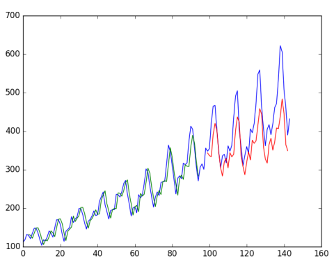
# plot baseline and predictions  
plt.plot(scaler.inverse_transform(dataset))  
plt.plot(trainPredictPlot)  
plt.plot(testPredictPlot)  
plt.show()

Run the above example to get the following output.

... 
Epoch 95/100 0s - loss: 0.0021 
Epoch 96/100 0s - loss: 0.0021 
Epoch 97/100 0s - loss: 0.0021 
Epoch 98/100 0s - loss: 0.0021 
Epoch 99/100 0s - loss: 0.0022 
Epoch 100/100 0s - loss: 0.0020 
Train Score: 24.19 RMSE 
Test Score: 58.03 RMSE

We can see a slight increase in errors compared with those in the last lesson. The window size and network interface are not adjusted, but show how to solve the prediction problem.

3 LSTM For Regression with Time Steps

You may have noticed that data preprocessing for LSTM networks includes time steps. Some timing problems may have different time steps. For example, you already have physical machine measurement data that leads to failure points and point aggregation. Each accident is a sample, then the observed value of the accident is taken as the time step, and the observed variables are characterized. Time step provides another way to state timing problems. Like the example in the window above, we take the previous time step in the sequence as the input value to predict the output value of the next time.

On the contrary, we take the past observations as a separate output feature, so that we can take an output feature as a time step, which is indeed a more accurate problem architecture. We can also use the same data representation in the previous window based example to do this, unless when we reorganize the data, we set this column as the time step dimension and change the feature dimension to 1. For example:

# reshape input to be [samples, time steps, features] 
trainX = numpy.reshape(trainX, (trainX.shape[0], trainX.shape[1], 1)) 
testX = numpy.reshape(testX, (testX.shape[0], testX.shape[1], 1))

For completeness, the entire code is listed below.

# LSTM for international airline passengers problem with time step regression framing  
import math  
  
import matplotlib.pyplot as plt  
import numpy  
from keras.layers import Dense  
from keras.layers import LSTM  
from keras.models import Sequential  
from pandas import read_csv  
from sklearn.metrics import mean_squared_error  
from sklearn.preprocessing import MinMaxScaler  
  
  
# convert an array of values into a dataset matrix  
def create_dataset(dataset, look_back=1):  
    dataX, dataY = [], []  
    for i in range(len(dataset) - look_back - 1):  
        a = dataset[i:(i + look_back), 0]  
        dataX.append(a)  
        dataY.append(dataset[i + look_back, 0])  
    return numpy.array(dataX), numpy.array(dataY)  
  
  
# fix random seed for reproducibility  
numpy.random.seed(7)  
# load the dataset  
dataframe = read_csv('international-airline-passengers.csv', usecols=[1], engine='python',  
                     skipfooter=3)  
dataset = dataframe.values  
dataset = dataset.astype('float32')  
# normalize the dataset  
scaler = MinMaxScaler(feature_range=(0, 1))  
dataset = scaler.fit_transform(dataset)  
# split into train and test sets  
train_size = int(len(dataset) * 0.67)  
test_size = len(dataset) - train_size  
train, test = dataset[0:train_size, :], dataset[train_size:len(dataset), :]  
# reshape into X=t and Y=t+1  
look_back = 3  
trainX, trainY = create_dataset(train, look_back)  
testX, testY = create_dataset(test, look_back)  
# reshape input to be [samples, time steps, features]  
trainX = numpy.reshape(trainX, (trainX.shape[0], trainX.shape[1], 1))  
testX = numpy.reshape(testX, (testX.shape[0], testX.shape[1], 1))  
# create and fit the LSTM network  
model = Sequential()  
model.add(LSTM(4, input_shape=(look_back, 1)))  
model.add(Dense(1))  
model.compile(loss='mean_squared_error', optimizer='adam')  
model.fit(trainX, trainY, epochs=100, batch_size=1, verbose=2)  
  
# make predictions  
trainPredict = model.predict(trainX)  
testPredict = model.predict(testX)  
  
# invert predictions  
trainPredict = scaler.inverse_transform(trainPredict)  
trainY = scaler.inverse_transform([trainY])  
testPredict = scaler.inverse_transform(testPredict)  
testY = scaler.inverse_transform([testY])  
  
# calculate root mean squared error  
trainScore = math.sqrt(mean_squared_error(trainY[0], trainPredict[:, 0]))  
print('Train Score: %.2f RMSE' % (trainScore))  
testScore = math.sqrt(mean_squared_error(testY[0], testPredict[:, 0]))  
print('Test Score: %.2f RMSE' % (testScore))  
  
# shift train predictions for plotting  
trainPredictPlot = numpy.empty_like(dataset)  
trainPredictPlot[:, :] = numpy.nan  
trainPredictPlot[look_back:len(trainPredict) + look_back, :] = trainPredict  
  
# shift test predictions for plotting  
testPredictPlot = numpy.empty_like(dataset)  
testPredictPlot[:, :] = numpy.nan  
testPredictPlot[len(trainPredict) + (look_back * 2) + 1:len(dataset) - 1, :] = testPredict  
  
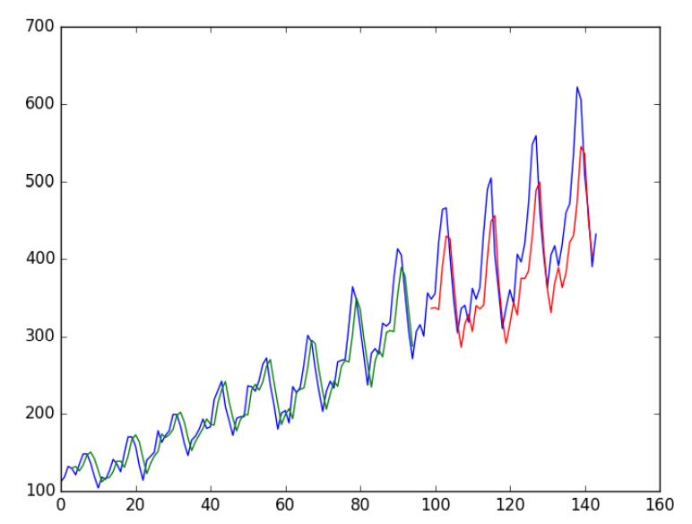
# plot baseline and predictions  
plt.plot(scaler.inverse_transform(dataset))  
plt.plot(trainPredictPlot)  
plt.plot(testPredictPlot)  
plt.show()

Run the above code to get the following results:

... 
Epoch 95/100 1s - loss: 0.0021 
Epoch 96/100 1s - loss: 0.0021 
Epoch 97/100 1s - loss: 0.0021 
Epoch 98/100 1s - loss: 0.0020 
Epoch 99/100 1s - loss: 0.0021 
Epoch 100/100 1s - loss: 0.0020 

Train Score: 23.69 RMSE 
Test Score: 58.88 RMSE

We can see that the result is slightly better than the previous example. The structure of the input data plays a role.

4 LSTM With Memory Between Batches.

LSTM network has memory function, which can remember the whole long sequence. Normally, when fitting the model, the status in the network will be reset after each batch training, and model.predict() or model.evaluate() will be called each time. When the LSTM network is cleared in Keras, we can make the LSTM layer stateful to obtain more accurate control. This means that he can build the state with the whole training sequence and maintain that state when we need to make predictions.

This requires that the training set cannot be disturbed when we fit the network, and it also needs to adjust model.reset after exposing the training set every time_ The states() function explicitly resets the network state. This means that you are calling model.fit() and model.reset_states() must create its own outer iteration loop. for instance:

for i in range(100): 
	model.fit(trainX, trainY, epochs=1, batch_size=batch_size, verbose=2, shuffle=False)
	model.reset_states()

Finally, when the LSTM layer is built, the stateful parameter must be set to True without specifying the input dimension. We use batch_ input_ The shape parameter passes in the number of batch samples, the number of time steps of samples and the number of features in time steps. for instance:

model.add(LSTM(4, batch_input_shape=(batch_size, time_steps, features), stateful=True))

When we evaluate models and make predictions, we must use the same batch size. For example:

model.predict(trainX, batch_size=batch_size)

The previous time step example is applicable to stateful LSTM. The complete code is provided below.

# LSTM for international airline passengers problem with memory  
import math  
  
import matplotlib.pyplot as plt  
import numpy  
from keras.layers import Dense  
from keras.layers import LSTM  
from keras.models import Sequential  
from pandas import read_csv  
from sklearn.metrics import mean_squared_error  
from sklearn.preprocessing import MinMaxScaler  
  
  
# convert an array of values into a dataset matrix  
def create_dataset(dataset, look_back=1):  
    dataX, dataY = [], []  
    for i in range(len(dataset) - look_back - 1):  
        a = dataset[i:(i + look_back), 0]  
        dataX.append(a)  
        dataY.append(dataset[i + look_back, 0])  
    return numpy.array(dataX), numpy.array(dataY)  
  
  
# fix random seed for reproducibility  
numpy.random.seed(7)  
# load the dataset  
dataframe = read_csv('international-airline-passengers.csv', usecols=[1], engine='python',  
                     skipfooter=3)  
dataset = dataframe.values  
dataset = dataset.astype('float32')  
# normalize the dataset  
scaler = MinMaxScaler(feature_range=(0, 1))  
dataset = scaler.fit_transform(dataset)  
# split into train and test sets  
train_size = int(len(dataset) * 0.67)  
test_size = len(dataset) - train_size  
train, test = dataset[0:train_size, :], dataset[train_size:len(dataset), :]  
# reshape into X=t and Y=t+1  
look_back = 3  
trainX, trainY = create_dataset(train, look_back)  
testX, testY = create_dataset(test, look_back)  
# reshape input to be [samples, time steps, features]  
trainX = numpy.reshape(trainX, (trainX.shape[0], trainX.shape[1], 1))  
testX = numpy.reshape(testX, (testX.shape[0], testX.shape[1], 1))  
# create and fit the LSTM network  
  
batch_size = 1  
model = Sequential()  
model.add(LSTM(4, batch_input_shape=(batch_size, look_back, 1), stateful=True))  
model.add(Dense(1))  
model.compile(loss='mean_squared_error', optimizer='adam')  
for i in range(100):  
    model.fit(trainX, trainY, epochs=1, batch_size=batch_size, verbose=2, shuffle=False)  
    model.reset_states()  
# make predictions  
trainPredict = model.predict(trainX, batch_size=batch_size)  
model.reset_states()  
testPredict = model.predict(testX, batch_size=batch_size)  
# invert predictions  
trainPredict = scaler.inverse_transform(trainPredict)  
trainY = scaler.inverse_transform([trainY])  
testPredict = scaler.inverse_transform(testPredict)  
testY = scaler.inverse_transform([testY])  
# calculate root mean squared error  
trainScore = math.sqrt(mean_squared_error(trainY[0], trainPredict[:, 0]))  
print('Train Score: %.2f RMSE' % (trainScore))  
testScore = math.sqrt(mean_squared_error(testY[0], testPredict[:, 0]))  
print('Test Score: %.2f RMSE' % (testScore))  
# shift train predictions for plotting  
trainPredictPlot = numpy.empty_like(dataset)  
trainPredictPlot[:, :] = numpy.nan  
trainPredictPlot[look_back:len(trainPredict) + look_back, :] = trainPredict  
# shift test predictions for plotting  
testPredictPlot = numpy.empty_like(dataset)  
testPredictPlot[:, :] = numpy.nan  
testPredictPlot[len(trainPredict) + (look_back * 2) + 1:len(dataset) - 1, :] = testPredict  
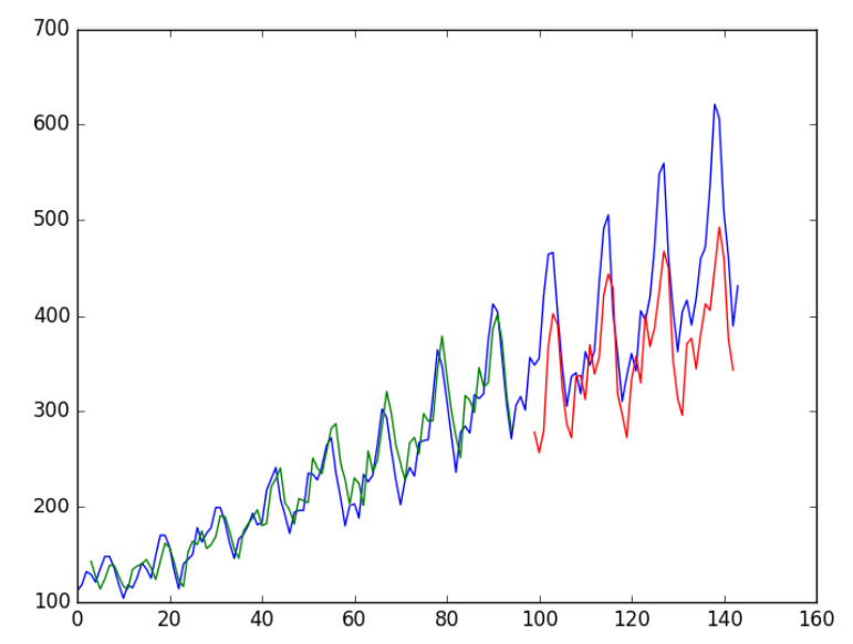
# plot baseline and predictions  
plt.plot(scaler.inverse_transform(dataset))  
plt.plot(trainPredictPlot)  
plt.plot(testPredictPlot)  
plt.show()

Run the above code and get the following results:

... 
Epoch 1/1 1s - loss: 0.0017 
Epoch 1/1 1s - loss: 0.0017 
Epoch 1/1 1s - loss: 0.0017 
Epoch 1/1 1s - loss: 0.0017 
Epoch 1/1 1s - loss: 0.0017 
Epoch 1/1 1s - loss: 0.0016 

Train Score: 20.74 RMSE 
Test Score: 52.23 RMSE

We can see that the results are better than some and worse than others. The model needs more modules and may need more iteration cycles to internalize some structural problems.

5 Stacked LSTMs With Memory Between Batches

Finally, we will look at one of the advantages of large lstms. When they are embedded in deep network structure, they can be successfully trained. LSTM network is embedded in Keras in the same way, and other types of layers can also be embedded. Another necessary configuration is that the LSTM layer before the LSTM layer must return this sequence. You can set return in the layer_ The sequences parameter is True. In the last part, we extended stateful LSTM, which has two layers, as follows:

model.add(LSTM(4, batch_input_shape=(batch_size, look_back, 1), stateful=True, return_sequences=True)) 
model.add(LSTM(4, batch_input_shape=(batch_size, look_back, 1), stateful=True))

For completeness, the whole code is given below.

# Stacked LSTM for international airline passengers problem with memory  
import math  
  
import matplotlib.pyplot as plt  
import numpy  
from keras.layers import Dense  
from keras.layers import LSTM  
from keras.models import Sequential  
from pandas import read_csv  
from sklearn.metrics import mean_squared_error  
from sklearn.preprocessing import MinMaxScaler  
  
  
# convert an array of values into a dataset matrix  
def create_dataset(dataset, look_back=1):  
    dataX, dataY = [], []  
    for i in range(len(dataset) - look_back - 1):  
        a = dataset[i:(i + look_back), 0]  
        dataX.append(a)  
        dataY.append(dataset[i + look_back, 0])  
    return numpy.array(dataX), numpy.array(dataY)  
  
  
# fix random seed for reproducibility  
numpy.random.seed(7)  

# load the dataset  
dataframe = read_csv('international-airline-passengers.csv', usecols=[1], engine='python',  
                     skipfooter=3)  
dataset = dataframe.values  
dataset = dataset.astype('float32')  

# normalize the dataset  
scaler = MinMaxScaler(feature_range=(0, 1))  
dataset = scaler.fit_transform(dataset)  

# split into train and test sets  
train_size = int(len(dataset) * 0.67)  
test_size = len(dataset) - train_size  
train, test = dataset[0:train_size, :], dataset[train_size:len(dataset), :]  

# reshape into X=t and Y=t+1  
look_back = 3  
trainX, trainY = create_dataset(train, look_back)  
testX, testY = create_dataset(test, look_back)  
# reshape input to be [samples, time steps, features]  
trainX = numpy.reshape(trainX, (trainX.shape[0], trainX.shape[1], 1))  
testX = numpy.reshape(testX, (testX.shape[0], testX.shape[1], 1))  

# create and fit the LSTM network  
batch_size = 1  
model = Sequential()  
model.add(LSTM(4, batch_input_shape=(batch_size, look_back, 1), stateful=True,  
               return_sequences=True))  
model.add(LSTM(4, batch_input_shape=(batch_size, look_back, 1), stateful=True))  
model.add(Dense(1))  
model.compile(loss='mean_squared_error', optimizer='adam')  
for i in range(100):  
    model.fit(trainX, trainY, epochs=1, batch_size=batch_size, verbose=2, shuffle=False)  
model.reset_states()  

# make predictions  
trainPredict = model.predict(trainX, batch_size=batch_size)  
model.reset_states()  
testPredict = model.predict(testX, batch_size=batch_size)  
# invert predictions  
trainPredict = scaler.inverse_transform(trainPredict)  
trainY = scaler.inverse_transform([trainY])  
testPredict = scaler.inverse_transform(testPredict)  
testY = scaler.inverse_transform([testY])  

# calculate root mean squared error  
trainScore = math.sqrt(mean_squared_error(trainY[0], trainPredict[:, 0]))  
print('Train Score: %.2f RMSE' % (trainScore))  
testScore = math.sqrt(mean_squared_error(testY[0], testPredict[:, 0]))  
print('Test Score: %.2f RMSE' % (testScore))  

# shift train predictions for plotting  
trainPredictPlot = numpy.empty_like(dataset)  
trainPredictPlot[:, :] = numpy.nan  
trainPredictPlot[look_back:len(trainPredict) + look_back, :] = trainPredict  

# shift test predictions for plotting  
testPredictPlot = numpy.empty_like(dataset)  
testPredictPlot[:, :] = numpy.nan  
testPredictPlot[len(trainPredict) + (look_back * 2) + 1:len(dataset) - 1, :] = testPredict  

# plot baseline and predictions  
plt.plot(scaler.inverse_transform(dataset))  
plt.plot(trainPredictPlot)  
plt.plot(testPredictPlot)  
plt.show()

Run the above code and get the following results:

... 
Epoch 1/1 1s - loss: 0.0017 
Epoch 1/1 1s - loss: 0.0017 
Epoch 1/1 1s - loss: 0.0017 
Epoch 1/1 1s - loss: 0.0017 
Epoch 1/1 1s - loss: 0.0016 

Train Score: 20.49 RMSE
Test Score: 56.35 RMSE

The predictions on the data set are getting worse again. Once again, there is evidence that we need additional training cycles.

summary

In this lesson, you have learned how to develop LSTM recurrent neural network to solve timing problems. In particular, you have learned about the timing prediction of international air passengers.

How to create an LSTM for the window format of regression and timing problems.
How to create LSTM in time step form of timing problem.
How to create LSTM network with state and embedded LSTM unit with state to learn long time series.

next step

In this lesson, you have learned how to use LSTM recurrent neural network to solve the problem of time series prediction. Next, you will use the new skills of discovering LSTM network to solve the problem of time series classification.

Keywords: AI neural networks Deep Learning lstm

Added by LTJason on Wed, 17 Nov 2021 05:13:51 +0200

Programming VIP