Pandas is an open source, BSD licensed library that must be mastered when starting Python to do data analysis. It provides high-performance, easy-to-use data structures and data analysis tools. The main data structures are Series (one-dimensional data) and DataFrame (two-dimensional data), which are sufficient to deal with most typical use cases in the fields of finance, statistics, social science, engineering and so on. Come and study together today.

Exercise 6 - Statistics
Explore wind speed data
- Step 1: import the necessary Libraries
# Run the following code
import pandas as pd
import datetime
- Step 2: import data from the following address
import pandas as pd
# Run the following code
path6 = "../input/pandas_exercise/pandas_exercise/exercise_data/wind.data"  # wind.data
- Step 3: store the data and set the first three columns as appropriate indexes
import datetime
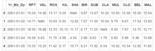
# Run the following code
data = pd.read_table(path6, sep = "\s+", parse_dates = [[0,1,2]])
data.head()
- Step 4: 2061? Do we really have data for this year? Create a function and use it to fix the bug
# Run the following code
def fix_century(x):
year = x.year - 100 if x.year > 1989 else x.year
return datetime.date(year, x.month, x.day)
# apply the function fix_century on the column and replace the values to the right ones
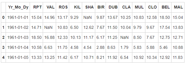
data['Yr_Mo_Dy'] = data['Yr_Mo_Dy'].apply(fix_century)
# data.info()
data.head()
- Step 5: set the date as the index. Note that the data type should be datetime64[ns]
# Run the following code
# transform Yr_Mo_Dy it to date type datetime64
data["Yr_Mo_Dy"] = pd.to_datetime(data["Yr_Mo_Dy"])
# set 'Yr_Mo_Dy' as the index
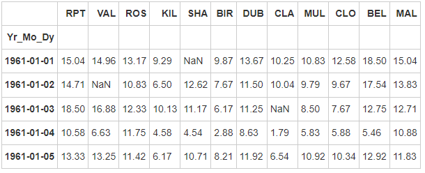
data = data.set_index('Yr_Mo_Dy')
data.head()
# data.info()
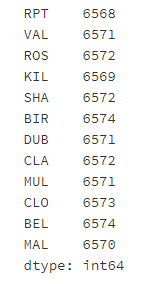
- Step 6: how many data values are missing for each location
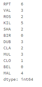
# Run the following code
data.isnull().sum()
- Step 7: how many complete data values are there for each location
# Run the following code
data.shape[0] - data.isnull().sum()
- Step 8: for all data, calculate the average value of wind speed
# Run the following code
data.mean().mean()
10.227982360836924
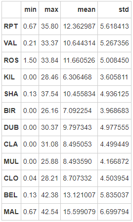
- Step 9: create a file named loc_stats data frame to calculate and store the minimum, maximum, average and standard deviation of wind speed at each location
# Run the following code
loc_stats = pd.DataFrame()

loc_stats['min'] = data.min() # min
loc_stats['max'] = data.max() # max
loc_stats['mean'] = data.mean() # mean
loc_stats['std'] = data.std() # standard deviations

loc_stats
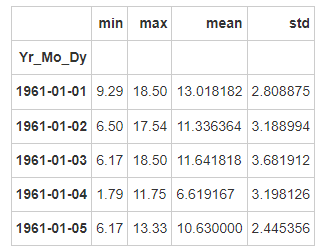
- Step 10: create a named day_stats data frame to calculate and store the minimum, maximum, average and standard deviation of wind speed at all location s
# Run the following code
# create the dataframe
day_stats = pd.DataFrame()

# this time we determine axis equals to one so it gets each row.
day_stats['min'] = data.min(axis = 1) # min
day_stats['max'] = data.max(axis = 1) # max
day_stats['mean'] = data.mean(axis = 1) # mean
day_stats['std'] = data.std(axis = 1) # standard deviations

day_stats.head()
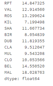
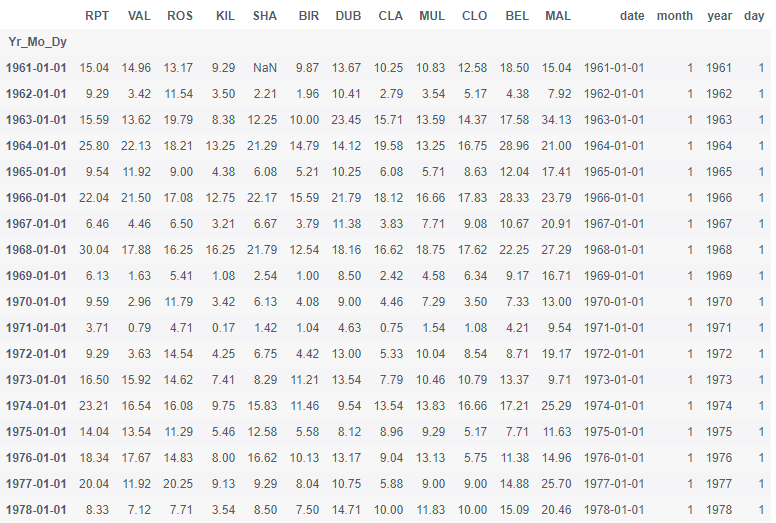
- Step 11: for each location, calculate the average wind speed in January
Note: January 1961 and January 1962 should be treated differently
# Run the following code
# creates a new column 'date' and gets the values from the index
data['date'] = data.index

# creates a column for each value from date
data['month'] = data['date'].apply(lambda date: date.month)
data['year'] = data['date'].apply(lambda date: date.year)
data['day'] = data['date'].apply(lambda date: date.day)

# gets all value from the month 1 and assign to janyary_winds
january_winds = data.query('month == 1')

# gets the mean from january_winds, using .loc to not print the mean of month, year and day
january_winds.loc[:,'RPT':"MAL"].mean()
- Step 12: for data records, take samples at the frequency of year
# Run the following code
data.query('month == 1 and day == 1')
- Step 13: for data records, the sampling frequency shall be monthly
# Run the following code
data.query('day == 1')
Exercise 7 - visualization
Explore Titanic disaster data
- Step 1: import the necessary Libraries
# Run the following code
import pandas as pd
import matplotlib.pyplot as plt
import seaborn as sns
import numpy as np

%matplotlib inline
- Step 2: import data from the following address
# Run the following code
path7 = '../input/pandas_exercise/pandas_exercise/exercise_data/train.csv'  # train.csv
- Step 3: name the data frame titanic
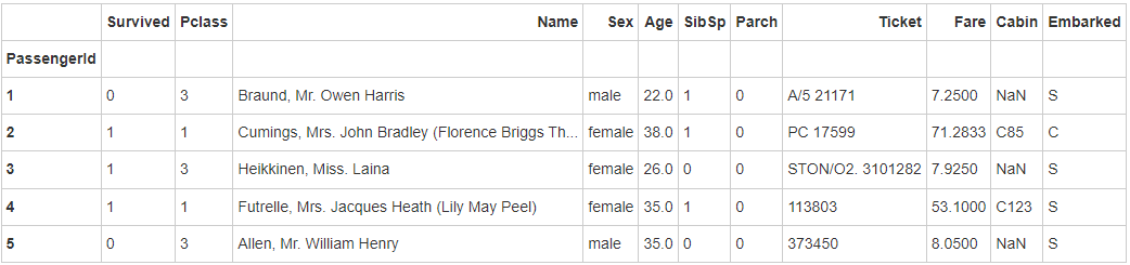
# Run the following code
titanic = pd.read_csv(path7)
titanic.head()
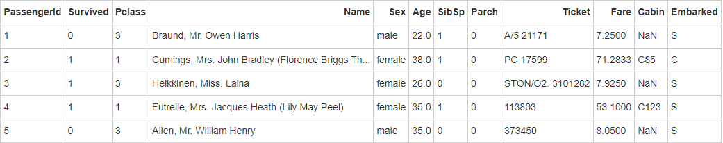
- Step 4: set the PassengerId as the index
# Run the following code
titanic.set_index('PassengerId').head()
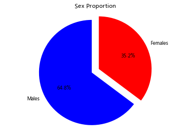
- Step 5: draw a sector chart showing the proportion of male and female passengers
# Run the following code
# sum the instances of males and females
males = (titanic['Sex'] == 'male').sum()
females = (titanic['Sex'] == 'female').sum()

# put them into a list called proportions
proportions = [males, females]

# Create a pie chart
plt.pie(
    # using proportions
    proportions,

    # with the labels being officer names
    labels = ['Males', 'Females'],

    # with no shadows
    shadow = False,

    # with colors
    colors = ['blue','red'],

    # with one slide exploded out
    explode = (0.15 , 0),

    # with the start angle at 90%
    startangle = 90,

    # with the percent listed as a fraction
    autopct = '%1.1f%%'
    )

# View the plot drop above
plt.axis('equal')

# Set labels
plt.title("Sex Proportion")

# View the plot
plt.tight_layout()
plt.show()
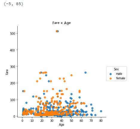
- Step 6: draw a scatter diagram showing Fare, age and gender of passengers
# Run the following code
# creates the plot using
lm = sns.lmplot(x = 'Age', y = 'Fare', data = titanic, hue = 'Sex', fit_reg=False)

# set title
lm.set(title = 'Fare x Age')

# get the axes object and tweak it
axes = lm.axes
axes[0,0].set_ylim(-5,)
axes[0,0].set_xlim(-5,85)
(-5, 85)
- Step 7: how many people are still alive?
# Run the following code
titanic.Survived.sum()
342
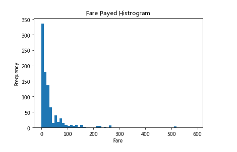
- Step 8: draw a histogram showing the ticket price
# Run the following code
# sort the values from the top to the least value and slice the first 5 items
df = titanic.Fare.sort_values(ascending = False)
df

# create bins interval using numpy
binsVal = np.arange(0,600,10)
binsVal

# create the plot
plt.hist(df, bins = binsVal)

# Set the title and labels
plt.xlabel('Fare')
plt.ylabel('Frequency')
plt.title('Fare Payed Histrogram')

# show the plot
plt.show()
Exercise 8 - creating a data frame
Explore Pokemon data
- Step 1: import the necessary Libraries
# Run the following code
import pandas as pd
- Step 2: create a data dictionary
# Run the following code
raw_data = {"name": ['Bulbasaur', 'Charmander','Squirtle','Caterpie'],
            "evolution": ['Ivysaur','Charmeleon','Wartortle','Metapod'],
            "type": ['grass', 'fire', 'water', 'bug'],
            "hp": [45, 39, 44, 45],
            "pokedex": ['yes', 'no','yes','no']
            }
- Step 3: save the data dictionary as a data box named pokemon
# Run the following code
pokemon = pd.DataFrame(raw_data)
pokemon.head()
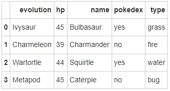
- Step 4: the columns of the data frame are sorted alphabetically. Please change the order to name, type, HP, evolution and pokedex
# Run the following code
pokemon = pokemon[['name', 'type', 'hp', 'evolution','pokedex']]
pokemon
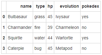
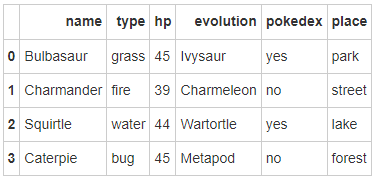
- Step 5: add a column place
# Run the following code
pokemon['place'] = ['park','street','lake','forest']
pokemon
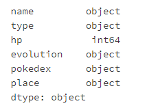
- Step 6: view the data type of each column
# Run the following code
pokemon.dtypes
Exercise 9 - time series
Explore Apple stock price data
- Step 1: import the necessary Libraries
# Run the following code
import pandas as pd
import numpy as np

# visualization
import matplotlib.pyplot as plt

%matplotlib inline
- Step 2: dataset address
# Run the following code
path9 = '../input/pandas_exercise/pandas_exercise/exercise_data/Apple_stock.csv'   # Apple_stock.csv
- Step 3: the read data coexists into a data frame called apple
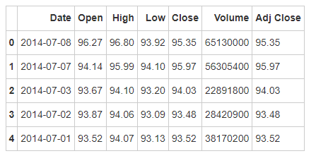
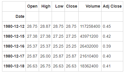
# Run the following code
apple = pd.read_csv(path9)
apple.head()
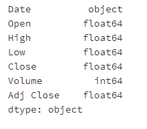
- Step 4: view the data type of each column
# Run the following code
apple.dtypes
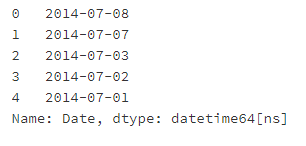
- Step 5: convert the Date column to the datetime type
# Run the following code
apple.Date = pd.to_datetime(apple.Date)
apple['Date'].head()
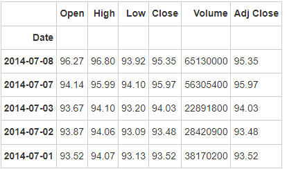
- Step 6: set Date as index
# Run the following code
apple = apple.set_index('Date')
apple.head()
- Step 7: is there a duplicate date?
# Run the following code
apple.index.is_unique
True
- Step 8: set index to ascending order
# Run the following code
apple.sort_index(ascending = True).head()
- Step 9: find the last business day of each month
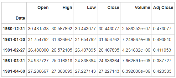
# Run the following code
apple_month = apple.resample('BM')
apple_month.head()
- Step 10 how many days is the difference between the earliest date and the latest date in the dataset?
# Run the following code
(apple.index.max() - apple.index.min()).days
12261
- Step 11: how many months are there in the data in step 11?
# Run the following code
apple_months = apple.resample('BM').mean()
len(apple_months.index)
404
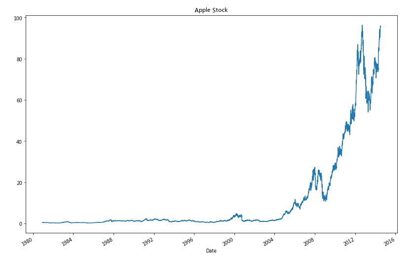
- Step 12: visualize Adj Close values in chronological order
# Run the following code
# makes the plot and assign it to a variable
appl_open = apple['Adj Close'].plot(title = "Apple Stock")

# changes the size of the graph
fig = appl_open.get_figure()
fig.set_size_inches(13.5, 9)
Exercise 10 - delete data
Explore Iris iris Iris data
- Step 1: import the necessary Libraries
# Run the following code
import pandas as pd
- Step 2: dataset address
# Run the following code
path10 ='../input/pandas_exercise/pandas_exercise/exercise_data/iris.csv'   # iris.csv
- Step 3: save the data set as the variable iris
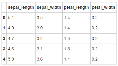
# Run the following code
iris = pd.read_csv(path10)
iris.head()
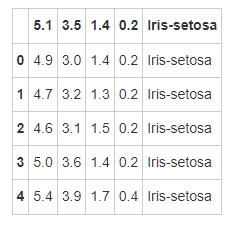
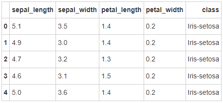
- Step 4: create the column name of the data frame
iris = pd.read_csv(path10,names = ['sepal_length','sepal_width', 'petal_length', 'petal_width', 'class'])
iris.head()
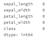
- Step 5: is there a missing value in the data frame?
# Run the following code
pd.isnull(iris).sum()
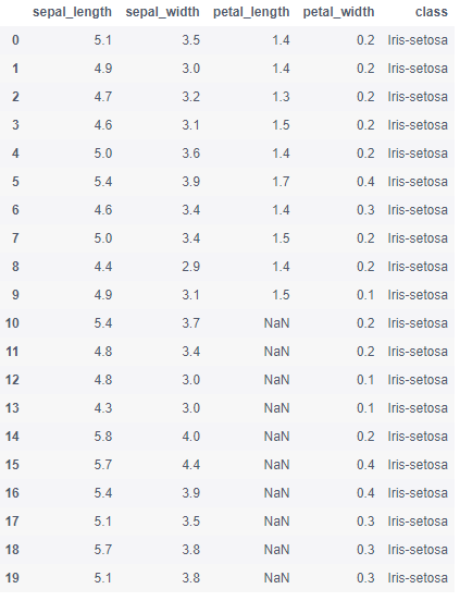
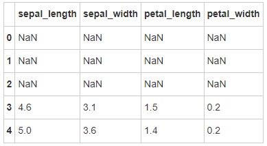
- Step 6: set the column petal_ Lines 10 to 19 of length are set to missing values
# Run the following code
iris.iloc[10:20,2:3] = np.nan
iris.head(20)
- Step 7: replace all missing values with 1.0
# Run the following code
iris.petal_length.fillna(1, inplace = True)
iris
- Step 8: delete column class
# Run the following code
del iris['class']
iris.head()
- Step 9: set the first three rows of the data frame as missing values
# Run the following code
iris.iloc[0:3 ,:] = np.nan
iris.head()
- Step 10: delete the row with missing value
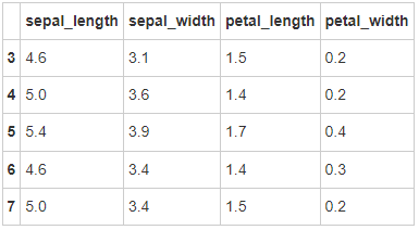
# Run the following code
iris = iris.dropna(how='any')
iris.head()
- Step 11: reset the index
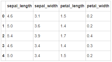
# Run the following code
iris = iris.reset_index(drop = True)
iris.head()
 Your support is the driving force for me to keep updating, (like, follow, comment) this article is not over yet. If you want to know about the follow-up, you can follow me and keep updating.

Click to receive 🎁🎁 Q group number: 943192807 (pure technical exchange and resource sharing) take it away by self-service.
① Industry consultation and professional answers ② Python development environment installation tutorial ③ 400 self-study videos ④ common vocabulary of software development ⑤ latest learning roadmap ⑥ more than 3000 Python e-books