Game address portal:
CCF big data and computing intelligence competition
First read the data
import matplotlib.pyplot as plt
import seaborn as sns
import gc
import re
import pandas as pd
import lightgbm as lgb
import numpy as np
from sklearn.metrics import roc_auc_score, precision_recall_curve, roc_curve, average_precision_score
from sklearn.model_selection import KFold
from lightgbm import LGBMClassifier
import matplotlib.pyplot as plt
import seaborn as sns
import gc
from sklearn.model_selection import StratifiedKFold
from dateutil.relativedelta import relativedelta
from sklearn.preprocessing import OneHotEncoder
train_data = pd.read_csv(r'data/data117603/train_public.csv')
test_public = pd.read_csv(r'data/data117603/test_public.csv')
df_features = train_data.append(test_public)
Try not to process the data first. What is the score of directly input into the model
LabelEncoder the text features first
cat_cols = ['class', 'employer_type', 'industry', 'work_year', 'issue_date', 'earlies_credit_mon']

from sklearn.preprocessing import LabelEncoder
for feat in cat_cols:
    lbl = LabelEncoder()
    df_features[feat] = lbl.fit_transform(df_features[feat])
lgb classification model is used for prediction
df_train = df_features[~df_features['isDefault'].isnull()]
df_train = df_train.reset_index(drop=True)
df_test = df_features[df_features['isDefault'].isnull()]

no_features = ['user_id', 'loan_id', 'isDefault']

# Input characteristic column
features = [col for col in df_train.columns if col not in no_features]

X = df_train[features] # Training set input
y = df_train['isDefault'] # Training set label
X_test = df_test[features] # Test set input
folds = KFold(n_splits=5, shuffle=True, random_state=2019)

oof_preds = np.zeros(X.shape[0])
sub_preds = np.zeros(X_test.shape[0])

for n_fold, (trn_idx, val_idx) in enumerate(folds.split(X)):
    trn_x, trn_y = X[features].iloc[trn_idx], y.iloc[trn_idx]
    val_x, val_y = X[features].iloc[val_idx], y.iloc[val_idx]
    clf = LGBMClassifier()

    clf.fit(trn_x, trn_y,
            eval_set= [(trn_x, trn_y), (val_x, val_y)],
            eval_metric='auc', verbose=100, early_stopping_rounds=40  #30
           )

    oof_preds[val_idx] = clf.predict_proba(val_x, num_iteration=clf.best_iteration_)[:, 1]
    sub_preds += clf.predict_proba(X_test[features], num_iteration=clf.best_iteration_)[:, 1] / folds.n_splits


    print('Fold %2d AUC : %.6f' % (n_fold + 1, roc_auc_score(val_y, oof_preds[val_idx])))
    del clf, trn_x, trn_y, val_x, val_y

print('Full AUC score %.6f' % roc_auc_score(y, oof_preds))
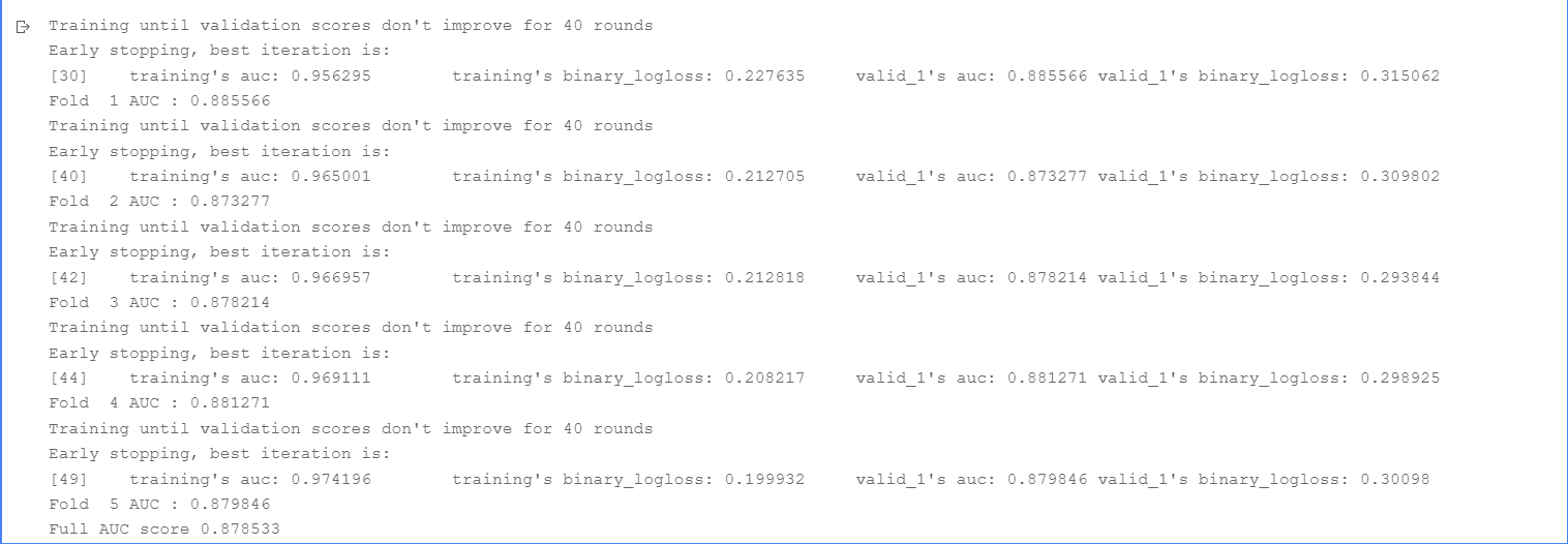
It can be seen here that when I only use LabelEncoder for text features, the AUC score is only 0.878533
Next, try to process the data
Because in 'work_ There are some features < 1 + 10 + in 'year', so I'll deal with these unqualified features first
def workYearDIc(x):
    if str(x)=='nan':
        return -1
    try:
        x = x.replace('< 1','0').replace('10+ ','10')
    except:
        pass
    return int(re.search('(\d+)', x).group())

df_features['work_year'] = df_features['work_year'].map(workYearDIc)
Next, I will deal with the characteristics of time according to the characteristics themselves
a = []
for i in range(15000):
    try:
        a.append(pd.to_datetime(df_features['earlies_credit_mon'].values[i]))
    except:
        try:
            a.append(pd.to_datetime('9' + df_features['earlies_credit_mon'].values[i]))
        except:
            a.append(pd.to_datetime('20' + df_features['earlies_credit_mon'].values[i]))

df_features['earlies_credit_mon'] = a

df_features['earlies_credit_mon'] = pd.to_datetime(df_features['earlies_credit_mon'])
df_features['issue_date'] = pd.to_datetime(df_features['issue_date'])
df_features['issue_date_month'] = df_features['issue_date'].dt.month
df_features['issue_date_dayofweek'] = df_features['issue_date'].dt.dayofweek
df_features['earliesCreditMon'] = df_features['earlies_credit_mon'].dt.month
df_features['earliesCreditYear'] = df_features['earlies_credit_mon'].dt.year
Identify category features
df_features['class'] = df_features['class'].map({'A': 0, 'B': 1, 'C': 2, 'D': 3, 'E': 4, 'F': 5, 'G': 6})
LabelEncoder the two features
cat_cols = ['employer_type', 'industry']

from sklearn.preprocessing import LabelEncoder
for col in cat_cols:
    lbl = LabelEncoder()
    df_features[col] = lbl.fit_transform(df_features[col])
Then delete the two previously processed features, and the feature 'policy_code 'because its values are all zero, it is also deleted
col_to_drop = ['issue_date', 'earlies_credit_mon', 'policy_code']
df_features = df_features.drop(col_to_drop, axis=1)
Then fill in some features with missing values * * -1**
df_features['pub_dero_bankrup'].fillna(-1, inplace=True)
df_features['f0'].fillna(-1, inplace=True)
df_features['f1'].fillna(-1, inplace=True)
df_features['f2'].fillna(-1, inplace=True)
df_features['f3'].fillna(-1, inplace=True)
df_features['f4'].fillna(-1, inplace=True)
Then divide the training and test sets
df_train = df_features[~df_features['isDefault'].isnull()]
df_train = df_train.reset_index(drop=True)
df_test = df_features[df_features['isDefault'].isnull()]

no_features = ['user_id', 'loan_id', 'isDefault']

# Input characteristic column
features = [col for col in df_train.columns if col not in no_features]

X = df_train[features] # Training set input
y = df_train['isDefault'] # Training set label
X_test = df_test[features] # Test set input
After that, the training set and test set are standardized. Here, I tried the maximum normalization and mean variance normalization, and found that the mean variance normalization is better, so I used the mean variance normalization
class StandardScaler:
    def __init__(self):
        self.mean_ = None
        self.scale_ = None
    def fit(self,X):
        '''According to the training data set X Obtain the mean and variance of the data'''
        self.mean_ = np.array([np.mean(X[:,i]) for i in range(X.shape[1])])
        self.scale_ = np.array([np.std(X[:,i]) for i in range(X.shape[1])])
        return self
    def transform(self,X):
        '''take X according to Standardcaler Normalize the mean variance'''
        resX = np.empty(shape=X.shape,dtype=float)
        for col in range(X.shape[1]):
            resX[:,col] = (X[:,col]-self.mean_[col]) / (self.scale_[col])
        return resX
X_col = X.columns
X_test_col = X_test.columns
StandardScaler = StandardScaler()
StandardScaler.fit(X.values)
X = StandardScaler.transform(X.values)
X_test = StandardScaler.transform(X_test.values)

X = pd.DataFrame(X, columns=X_col)
X_test = pd.DataFrame(X_test, columns=X_test_col)
Because there is a problem of sample imbalance in this training set, I use SMOTE function for oversampling to solve the imbalance problem. It may be better to use down sampling or other methods to deal with sample imbalance here, but I haven't tried others. We can try others
from imblearn.over_sampling import SMOTE

X, y = SMOTE(random_state=42).fit_resample(X, y)
Next, input model training samples to see the effect
folds = KFold(n_splits=5, shuffle=True, random_state=2019)

oof_preds = np.zeros(X.shape[0])
sub_preds = np.zeros(X_test.shape[0])

for n_fold, (trn_idx, val_idx) in enumerate(folds.split(X)):
    trn_x, trn_y = X[features].iloc[trn_idx], y.iloc[trn_idx]
    val_x, val_y = X[features].iloc[val_idx], y.iloc[val_idx]
    clf = LGBMClassifier()

    clf.fit(trn_x, trn_y,
            eval_set= [(trn_x, trn_y), (val_x, val_y)],
            eval_metric='auc', verbose=100, early_stopping_rounds=40  #30
           )

    oof_preds[val_idx] = clf.predict_proba(val_x, num_iteration=clf.best_iteration_)[:, 1]
    sub_preds += clf.predict_proba(X_test[features], num_iteration=clf.best_iteration_)[:, 1] / folds.n_splits


    print('Fold %2d AUC : %.6f' % (n_fold + 1, roc_auc_score(val_y, oof_preds[val_idx])))
    del clf, trn_x, trn_y, val_x, val_y

print('Full AUC score %.6f' % roc_auc_score(y, oof_preds))
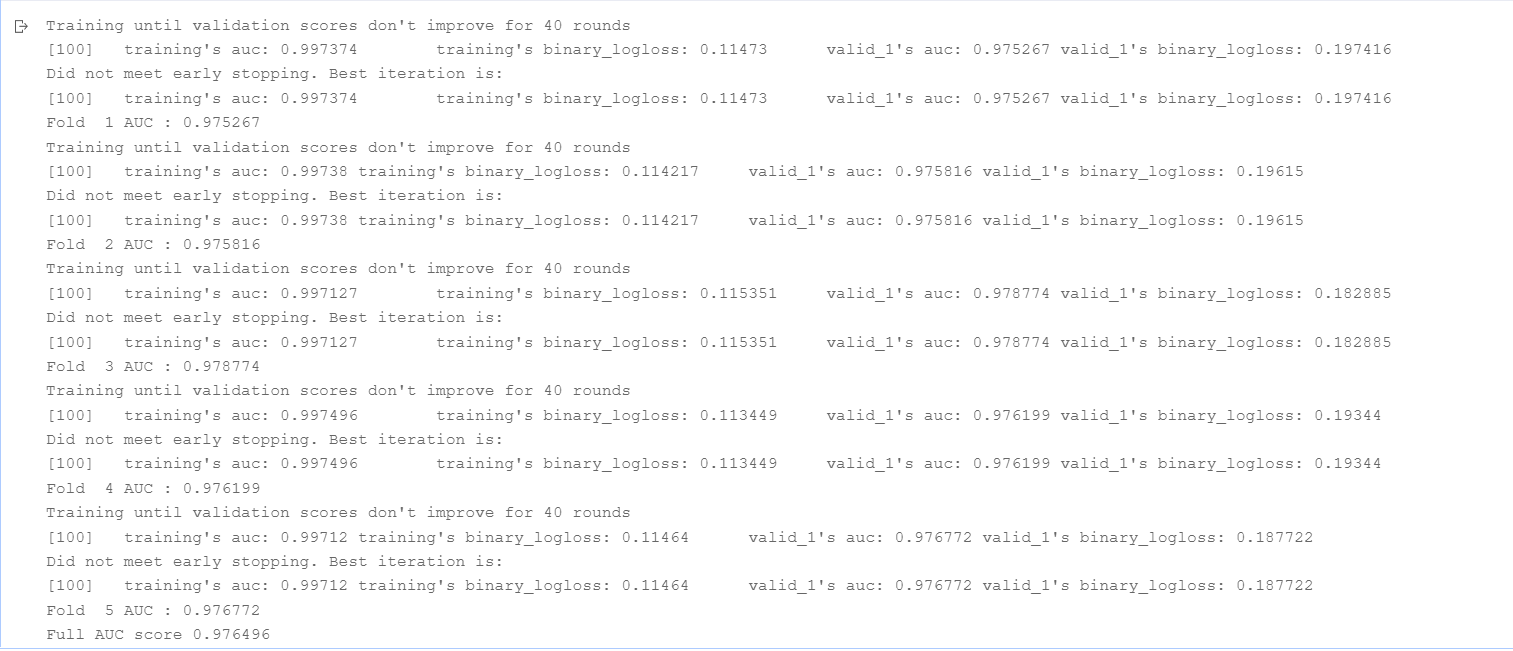
In the final results, it can be seen that the AUC score after feature processing has been greatly improved
Then we look at the correlation between features to construct some new features according to these correlations
The correlation between features is calculated and displayed by thermal diagram
from pylab import mpl
mpl.rcParams['font.sans-serif'] = ['FangSong'] # Specifies the default font
mpl.rcParams['axes.unicode_minus'] = False # Solve the problem that the saved image is negative
plt.figure(figsize=(30, 30))
ax = sns.heatmap(df_features.corr(),linewidths=5,vmax=1.0, square=True,linecolor='white', annot=True)
ax.tick_params(labelsize=10)
plt.show()
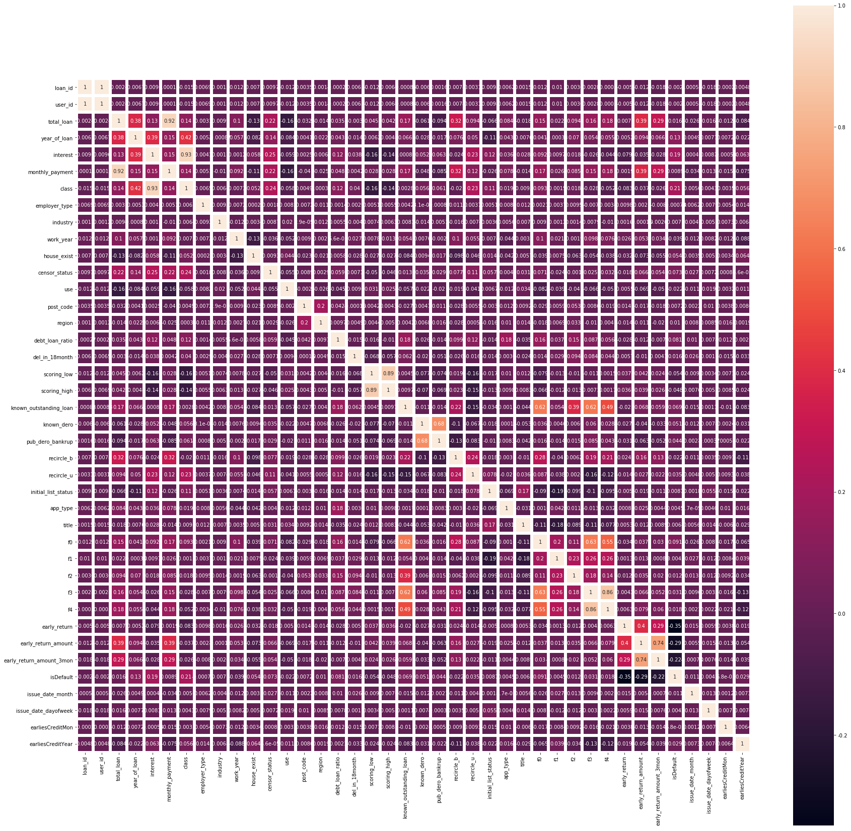
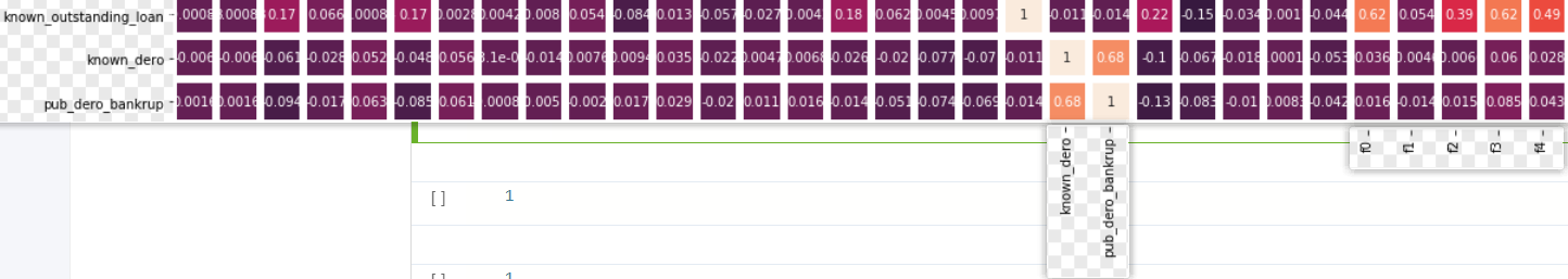
Looking at this thermodynamic diagram, it is not difficult for us to find a large correlation between some features


I have fused the features with high correlation between these features. I have tried many times and found that the following are the most important factors to improve the score
However, I tried one by one before. These new features are obvious for the improvement of AUC. However, when I added these new features to the model for training, I found that the improvement of AUC is not great, but I listed them and added them to the training together
df_features['new_1'] = df_features['total_loan'] / df_features['monthly_payment']
df_features['new_3'] = df_features['known_dero'] - df_features['pub_dero_bankrup']
df_features['new_6'] = df_features['known_outstanding_loan'] * df_features['pub_dero_bankrup']
df_features['new_11'] = df_features['f0'] / df_features['f3']
df_features['new_12'] = df_features['f0'] + df_features['f4']
df_features['new_18'] = df_features['f3'] * df_features['f4']
The final training scores are as follows:

Finally, we perform pseudo label processing on the data to further improve our AUC
Here is an introduction to pseudo tags
Here, I set all the data with the predicted value less than 0.05 to 0 and add it to the training set as a pseudo label, because the predicted result less than or equal to 0.05 can generally be regarded as 0
test_public['isDefault'] = sub_preds
test_public.loc[test_public['isDefault']<0.05,'isDefault'] = 0

InteId = test_public.loc[test_public.isDefault<0.05, 'loan_id'].tolist()
use_te = test_public[test_public.loan_id.isin( InteId )].copy()
Then re read the data of the training set and prediction set, and then combine the two data with the data we want to use as a pseudo label to form a new data
test = pd.read_csv(r'data/data117603/test_public.csv')
train = pd.read_csv(r'data/data117603/train_public.csv')
df_features = pd.concat([train,test,use_te]).reset_index(drop=True)
After that, as like as two peas, the character processing is then put into the model for training.
The training results are as follows:

From the results, we can see that the improvement is still very large,
In fact, many iterations can be carried out here to add more pseudo tags, but I won't do so many times here
Moreover, it would be better to rely on the business background for feature processing, but I didn't do data processing based on the business background because I didn't understand the business background