I've heard that many bosses acquire knowledge from kaggle and process it into their own competition system
In July this year, I started to participate in the big data competition. Now there are almost 10 competitions, all of which are structured competitions. Small competitions can still get into the Top ranking, but larger competitions are more difficult. The problem is that there is no system, so I plan to structure the kaggle. In the timing competition, I will simply translate and sort out the better notebook and summarize the useful information, I hope to have better results in the future competitions
Focus of this paper
Taking the Titanic competition data on kaggle as an example, this paper introduces how to integrate the stacking model. The number of likes on kaggle exceeds 5000. The original link: kaggle Titanic
After careful study, the following ideas can be used for reference:
Characteristic Engineering
- Classification features can be classified into 2 categories by whether they are missing values or not, and can also be filled into the largest number of categories
- Missing value filling method for numerical characteristic age
- Numerical equidistant and equifrequency discretization
- Text processing, some information in foreigners' names
Model
- A class sklearnhelp is created to improve code efficiency
- The first layer is five base models, and the second layer is xgboost (linear regression is also used in some articles)
- Each base model in layer 1 uses k-fold cross validation, outputs the predicted values of train and test, and then splices the data to construct a new train_new and test_new, label or original label
- Finally, the layer 2 model is trained with new data to output the final prediction value
# Import Toolkit
import pandas as pd
import numpy as np
import re
import sklearn
import xgboost as xgb
import seaborn as sns
import matplotlib.pyplot as plt
%matplotlib inline

import plotly.offline as py
py.init_notebook_mode(connected=True)
import plotly.graph_objs as go
import plotly.tools as tls

import warnings
warnings.filterwarnings('ignore')

# 5 basic models
from sklearn.ensemble import (RandomForestClassifier, AdaBoostClassifier,
                              GradientBoostingClassifier, ExtraTreesClassifier)
from sklearn.svm import SVC
from sklearn.cross_validation import KFold
Feature Engineering and processing
Like most other kernel structures, we first explore the data at hand, identify possible feature engineering, and digitize text features
# Import training data and test data
train = pd.read_csv('../input/train.csv')
test = pd.read_csv('../input/test.csv')

# Store passenger ID
PassengerId = test['PassengerId']

train.head(3)
There is no doubt that we will extract information from classification features
Characteristic Engineering
# Combined training data and test data
full_data = [train, test]

# Name length
train['Name_length'] = train['Name'].apply(len)
test['Name_length'] = test['Name'].apply(len)
# Does the passenger have a cabin number on board
train['Has_Cabin'] = train["Cabin"].apply(lambda x: 0 if type(x) == float else 1)
test['Has_Cabin'] = test["Cabin"].apply(lambda x: 0 if type(x) == float else 1)

# Combine SibSp and Parch features
for dataset in full_data:
    dataset['FamilySize'] = dataset['SibSp'] + dataset['Parch'] + 1
# Is it a person
for dataset in full_data:
    dataset['IsAlone'] = 0
    dataset.loc[dataset['FamilySize'] == 1, 'IsAlone'] = 1
# If the boarding port is empty, it is filled with class S
for dataset in full_data:
    dataset['Embarked'] = dataset['Embarked'].fillna('S')
#  The missing fare value is filled as the mean
for dataset in full_data:
    dataset['Fare'] = dataset['Fare'].fillna(train['Fare'].median())
# Ticket prices are discretized by Quantile
train['CategoricalFare'] = pd.qcut(train['Fare'], 4)
# Age missing value filling
for dataset in full_data:
    age_avg = dataset['Age'].mean()
    age_std = dataset['Age'].std()
    age_null_count = dataset['Age'].isnull().sum()
    age_null_random_list = np.random.randint(age_avg - age_std, age_avg + age_std, size=age_null_count)
    dataset['Age'][np.isnan(dataset['Age'])] = age_null_random_list
    dataset['Age'] = dataset['Age'].astype(int)
# Age is discretized by Quantile
train['CategoricalAge'] = pd.cut(train['Age'], 5)
# Define functions to handle passenger names
def get_title(name):
    title_search = re.search(' ([A-Za-z]+)\.', name)
    # If the title exists, extract and return it.
    if title_search:
        return title_search.group(1)
    return ""
# Create a new feature, called title
for dataset in full_data:
    dataset['Title'] = dataset['Name'].apply(get_title)
# Classify the uncommon as category 1 and replace the others
for dataset in full_data:
    dataset['Title'] = dataset['Title'].replace(['Lady', 'Countess','Capt', 'Col','Don', 'Dr', 'Major', 'Rev', 'Sir', 'Jonkheer', 'Dona'], 'Rare')

    dataset['Title'] = dataset['Title'].replace('Mlle', 'Miss')
    dataset['Title'] = dataset['Title'].replace('Ms', 'Miss')
    dataset['Title'] = dataset['Title'].replace('Mme', 'Mrs')

for dataset in full_data:
    # Gender numerical code
    dataset['Sex'] = dataset['Sex'].map( {'female': 0, 'male': 1} ).astype(int)

    # Encode the title value
    title_mapping = {"Mr": 1, "Miss": 2, "Mrs": 3, "Master": 4, "Rare": 5}
    dataset['Title'] = dataset['Title'].map(title_mapping)
    dataset['Title'] = dataset['Title'].fillna(0)

    # Numerical code of boarding port
    dataset['Embarked'] = dataset['Embarked'].map( {'S': 0, 'C': 1, 'Q': 2} ).astype(int)

    # Fare discretization
    dataset.loc[ dataset['Fare'] <= 7.91, 'Fare'] 						        = 0
    dataset.loc[(dataset['Fare'] > 7.91) & (dataset['Fare'] <= 14.454), 'Fare'] = 1
    dataset.loc[(dataset['Fare'] > 14.454) & (dataset['Fare'] <= 31), 'Fare']   = 2
    dataset.loc[ dataset['Fare'] > 31, 'Fare'] 							        = 3
    dataset['Fare'] = dataset['Fare'].astype(int)

    # Age discretization
    dataset.loc[ dataset['Age'] <= 16, 'Age'] 					       = 0
    dataset.loc[(dataset['Age'] > 16) & (dataset['Age'] <= 32), 'Age'] = 1
    dataset.loc[(dataset['Age'] > 32) & (dataset['Age'] <= 48), 'Age'] = 2
    dataset.loc[(dataset['Age'] > 48) & (dataset['Age'] <= 64), 'Age'] = 3
    dataset.loc[ dataset['Age'] > 64, 'Age'] = 4 ;
# feature selection
drop_elements = ['PassengerId', 'Name', 'Ticket', 'Cabin', 'SibSp']
# Delete the original text feature
train = train.drop(drop_elements, axis = 1)
# Delete 2 features created but not used (estimated to be used for viewing distribution)
train = train.drop(['CategoricalAge', 'CategoricalFare'], axis = 1)
test  = test.drop(drop_elements, axis = 1)
Now we clean and extract the relevant information, delete the text column, and all the features are numerical columns, which are suitable for the machine learning model. Before we continue, let's do some simple correlation and distribution diagrams
visualization
train.head(3)
Pearson correlation heat map
Generate correlation diagrams of some features to view the correlation between one feature and the next.
colormap = plt.cm.RdBu
plt.figure(figsize=(14,12))
plt.title('Pearson Correlation of Features', y=1.05, size=15)
sns.heatmap(train.astype(float).corr(),linewidths=0.1,vmax=1.0,
            square=True, cmap=colormap, linecolor='white', annot=True)
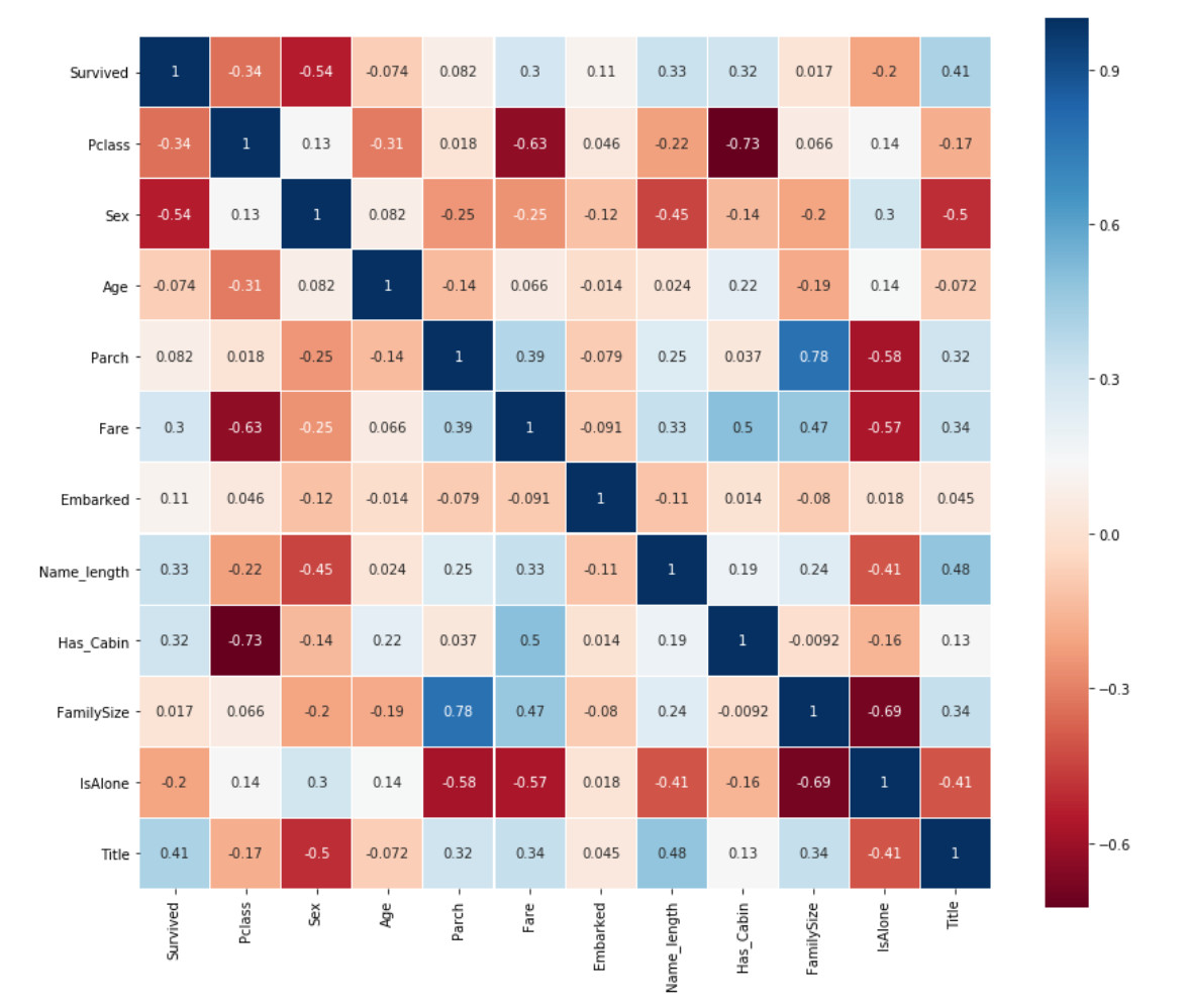
Get information from diagram
One thing Pearson correlation diagram can tell us is that not many features have a strong correlation with each other. From the perspective of inputting these functions into the learning model, this is good because it means that there is not much redundant or redundant data in our training set, and we are glad that each feature has some unique information. The two most relevant characteristics here are family size and Parch (parents and children). For the purposes of this exercise, I will retain these two features.
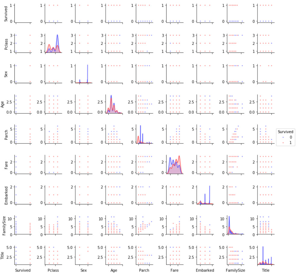
Pairplots
Finally, let's generate some pairing graphs to observe the distribution of data features
g = sns.pairplot(train[[u'Survived', u'Pclass', u'Sex', u'Age', u'Parch', u'Fare', u'Embarked',
       u'FamilySize', u'Title']], hue='Survived', palette = 'seismic',size=1.2,diag_kind = 'kde',diag_kws=dict(shade=True),plot_kws=dict(s=10) )
g.set(xticklabels=[])
Integration and integration model (stacking)
# Some parameters
ntrain = train.shape[0]
ntest = test.shape[0]
SEED = 0 # Reappearance
NFOLDS = 5 #
kf = KFold(ntrain, n_folds= NFOLDS, random_state=SEED)

# Create a machine learning extension class
class SklearnHelper(object):
    def __init__(self, clf, seed=0, params=None):
        params['random_state'] = seed
        self.clf = clf(**params)

    def train(self, x_train, y_train):
        self.clf.fit(x_train, y_train)

    def predict(self, x):
        return self.clf.predict(x)

    def fit(self,x,y):
        return self.clf.fit(x,y)

    def feature_importances(self,x,y):
        print(self.clf.fit(x,y).feature_importances_)

# Class to extend XGboost classifer
For those who already know this, please forgive me, but for those who have not created classes or objects in Python before, let me explain what the code given above does. When creating a basic classifier, I will only use models that already exist in the Sklearn library, so I will only extend this class.
Define init: the default constructor of the python standard calling class. This means that when you want to create an object (classifier), you must provide it with the parameters of clf (sklearn classifier you want), seed (random seed), and params (classifier parameters).
The rest of the code is just the methods of the class. They just call the corresponding methods that already exist in the sklearn classifier. In essence, we create an encapsulation class to extend various sklearn classifiers, so that when we implement multiple learners, we can reduce the number of times to write the same code repeatedly.
Out-of-Fold Predictions
Now, as mentioned in the introduction above, stacking uses the prediction of the basic classifier as the input of the second level model training. However, it is impossible to simply train the basic model based on the complete training data, generate predictions on the complete test set, and then output these predictions for the second level training. This will cause your underlying model predictions to "see" the test set, so there is a risk of over fitting when entering these predictions.
def get_oof(clf, x_train, y_train, x_test):
    oof_train = np.zeros((ntrain,))
    oof_test = np.zeros((ntest,))
    oof_test_skf = np.empty((NFOLDS, ntest))

    for i, (train_index, test_index) in enumerate(kf):
        x_tr = x_train[train_index]
        y_tr = y_train[train_index]
        x_te = x_train[test_index]

        clf.train(x_tr, y_tr)

        oof_train[test_index] = clf.predict(x_te)
        oof_test_skf[i, :] = clf.predict(x_test)

    oof_test[:] = oof_test_skf.mean(axis=0)
    return oof_train.reshape(-1, 1), oof_test.reshape(-1, 1)
# The code is actually very similar to page 89 of the book. It turns out that many of them are from kaggle
Generate layer 1 model
Now let's prepare five learning models as the first level classification. These models can be easily called through the Sklearn library, as shown below:
- Random Forest classifier
- Extra Trees classifier
- AdaBoost classifer
- Gradient Boosting classifer
- Support Vector Machine
parameter
For completeness, we will list a brief summary of the parameters here,
n_jobs: the number of jobs used by the kernel during training. If set to - 1, all jobs will be used
n_estimators: the number of classifiers in the learning model
max_depth: the maximum depth of the tree, or how much a node should expand. Note that if the number is set too high, there is a risk of over fitting
verbose: controls whether to output any text during the learning process. A value of 0 suppresses all text, while a value of 3 outputs the tree learning process at each iteration.
Please check the full description on the official Sklearn website. Here, you will find many other useful parameters that you can use.
# Enter the parameters of the classifier to which you belong
# Random Forest parameters
rf_params = {
    'n_jobs': -1,
    'n_estimators': 500,
     'warm_start': True,
     #'max_features': 0.2,
    'max_depth': 6,
    'min_samples_leaf': 2,
    'max_features' : 'sqrt',
    'verbose': 0
}

# Extra Trees Parameters
et_params = {
    'n_jobs': -1,
    'n_estimators':500,
    #'max_features': 0.5,
    'max_depth': 8,
    'min_samples_leaf': 2,
    'verbose': 0
}

# AdaBoost parameters
ada_params = {
    'n_estimators': 500,
    'learning_rate' : 0.75
}

# Gradient Boosting parameters
gb_params = {
    'n_estimators': 500,
     #'max_features': 0.2,
    'max_depth': 5,
    'min_samples_leaf': 2,
    'verbose': 0
}

# Support Vector Classifier parameters
svc_params = {
    'kernel' : 'linear',
    'C' : 0.025
    }
Furthermore, since having mentioned about Objects and classes within the OOP framework, let us now create 5 objects that represent our 5 learning models via our Helper Sklearn Class we defined earlier.
# Create 5 objects that represent our 4 models
rf = SklearnHelper(clf=RandomForestClassifier, seed=SEED, params=rf_params)
et = SklearnHelper(clf=ExtraTreesClassifier, seed=SEED, params=et_params)
ada = SklearnHelper(clf=AdaBoostClassifier, seed=SEED, params=ada_params)
gb = SklearnHelper(clf=GradientBoostingClassifier, seed=SEED, params=gb_params)
svc = SklearnHelper(clf=SVC, seed=SEED, params=svc_params)
Building arrays using training and test sets
After preparing the basic model of the first layer, we can now prepare the training and test data by generating a NumPy array from the original data for input to the classifier, as follows:
# Create Numpy arrays of train, test and target ( Survived) dataframes to feed into our models
y_train = train['Survived'].ravel()
train = train.drop(['Survived'], axis=1)
x_train = train.values # Creates an array of the train data
x_test = test.values # Creats an array of the test data
Output layer 1 forecast
Now, we input the training and test data into five base classifiers, and use the out of fold prediction function we defined earlier to generate our first layer prediction. Allow the following code block to run for a few minutes.
# Create training set and test set predictions
et_oof_train, et_oof_test = get_oof(et, x_train, y_train, x_test) # Extra Trees
rf_oof_train, rf_oof_test = get_oof(rf,x_train, y_train, x_test) # Random Forest
ada_oof_train, ada_oof_test = get_oof(ada, x_train, y_train, x_test) # AdaBoost
gb_oof_train, gb_oof_test = get_oof(gb,x_train, y_train, x_test) # Gradient Boost
svc_oof_train, svc_oof_test = get_oof(svc,x_train, y_train, x_test) # Support Vector Classifier

print("Training is complete")
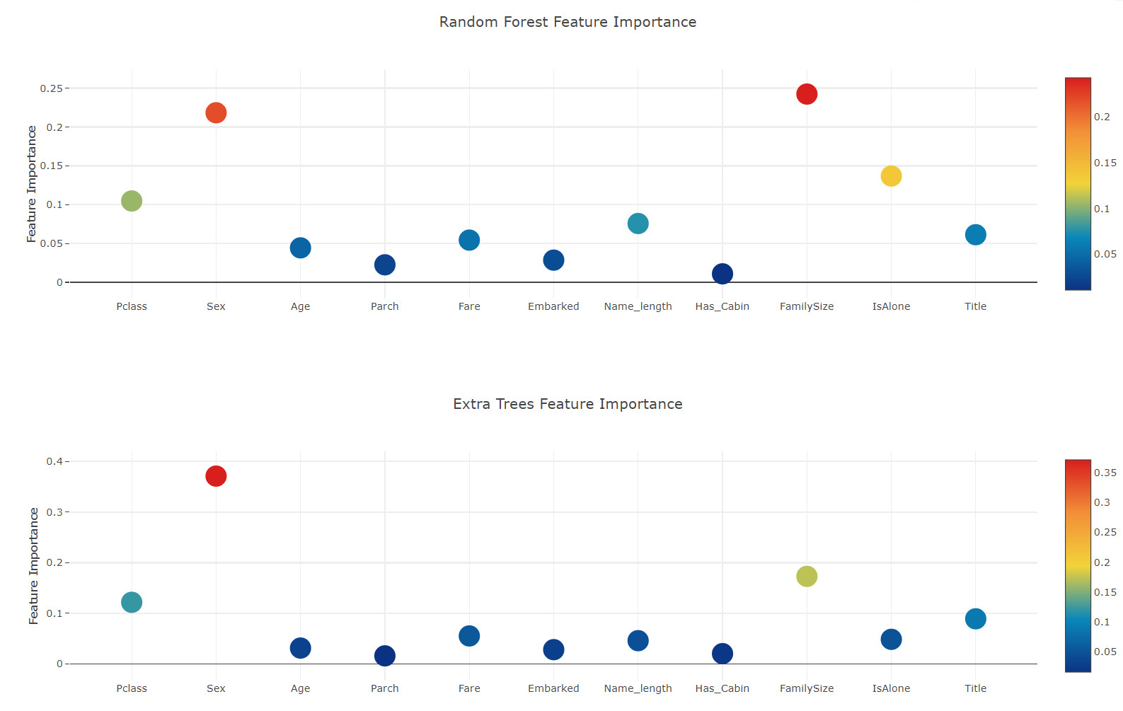
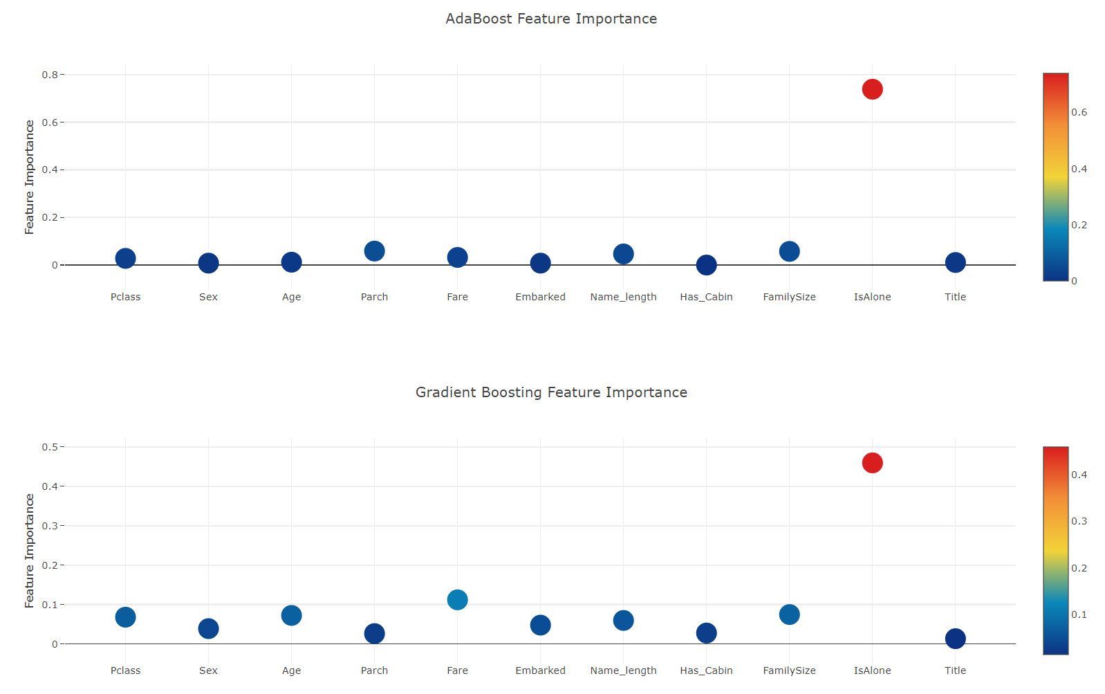
Feature importance generated from different classifiers
Now, after learning the first level classifier, we can take advantage of a very excellent function of Sklearn model, that is, to output the importance of various functions in the training set and test set with a very simple line of code.
According to the Sklearn document, most classifiers have a built-in attribute, which only needs to enter * *. feature_importances returns the functional importance. Therefore, we will call this very useful attribute through our function Earlian to draw the importance of the feature
rf_feature = rf.feature_importances(x_train,y_train)
et_feature = et.feature_importances(x_train, y_train)
ada_feature = ada.feature_importances(x_train, y_train)
gb_feature = gb.feature_importances(x_train,y_train)
rf_features = [0.10474135,  0.21837029,  0.04432652,  0.02249159,  0.05432591,  0.02854371
  ,0.07570305,  0.01088129 , 0.24247496,  0.13685733 , 0.06128402]
et_features = [ 0.12165657,  0.37098307  ,0.03129623 , 0.01591611 , 0.05525811 , 0.028157
  ,0.04589793 , 0.02030357 , 0.17289562 , 0.04853517,  0.08910063]
ada_features = [0.028 ,   0.008  ,      0.012   ,     0.05866667,   0.032 ,       0.008
  ,0.04666667 ,  0.     ,      0.05733333,   0.73866667,   0.01066667]
gb_features = [ 0.06796144 , 0.03889349 , 0.07237845 , 0.02628645 , 0.11194395,  0.04778854
  ,0.05965792 , 0.02774745,  0.07462718,  0.4593142 ,  0.01340093]
Create a dataframe
cols = train.columns.values
# Create a dataframe with features
feature_dataframe = pd.DataFrame( {'features': cols,
     'Random Forest feature importances': rf_features,
     'Extra Trees  feature importances': et_features,
      'AdaBoost feature importances': ada_features,
    'Gradient Boost feature importances': gb_features
    })
Determine the importance of interaction features by drawing scatter diagrams
# Scatter plot
trace = go.Scatter(
    y = feature_dataframe['Random Forest feature importances'].values,
    x = feature_dataframe['features'].values,
    mode='markers',
    marker=dict(
        sizemode = 'diameter',
        sizeref = 1,
        size = 25,
#       size= feature_dataframe['AdaBoost feature importances'].values,
        #color = np.random.randn(500), #set color equal to a variable
        color = feature_dataframe['Random Forest feature importances'].values,
        colorscale='Portland',
        showscale=True
    ),
    text = feature_dataframe['features'].values
)
data = [trace]

layout= go.Layout(
    autosize= True,
    title= 'Random Forest Feature Importance',
    hovermode= 'closest',
#     xaxis= dict(
#         title= 'Pop',
#         ticklen= 5,
#         zeroline= False,
#         gridwidth= 2,
#     ),
    yaxis=dict(
        title= 'Feature Importance',
        ticklen= 5,
        gridwidth= 2
    ),
    showlegend= False
)
fig = go.Figure(data=data, layout=layout)
py.iplot(fig,filename='scatter2010')

# Scatter plot
trace = go.Scatter(
    y = feature_dataframe['Extra Trees  feature importances'].values,
    x = feature_dataframe['features'].values,
    mode='markers',
    marker=dict(
        sizemode = 'diameter',
        sizeref = 1,
        size = 25,
#       size= feature_dataframe['AdaBoost feature importances'].values,
        #color = np.random.randn(500), #set color equal to a variable
        color = feature_dataframe['Extra Trees  feature importances'].values,
        colorscale='Portland',
        showscale=True
    ),
    text = feature_dataframe['features'].values
)
data = [trace]

layout= go.Layout(
    autosize= True,
    title= 'Extra Trees Feature Importance',
    hovermode= 'closest',
#     xaxis= dict(
#         title= 'Pop',
#         ticklen= 5,
#         zeroline= False,
#         gridwidth= 2,
#     ),
    yaxis=dict(
        title= 'Feature Importance',
        ticklen= 5,
        gridwidth= 2
    ),
    showlegend= False
)
fig = go.Figure(data=data, layout=layout)
py.iplot(fig,filename='scatter2010')

# Scatter plot
trace = go.Scatter(
    y = feature_dataframe['AdaBoost feature importances'].values,
    x = feature_dataframe['features'].values,
    mode='markers',
    marker=dict(
        sizemode = 'diameter',
        sizeref = 1,
        size = 25,
#       size= feature_dataframe['AdaBoost feature importances'].values,
        #color = np.random.randn(500), #set color equal to a variable
        color = feature_dataframe['AdaBoost feature importances'].values,
        colorscale='Portland',
        showscale=True
    ),
    text = feature_dataframe['features'].values
)
data = [trace]

layout= go.Layout(
    autosize= True,
    title= 'AdaBoost Feature Importance',
    hovermode= 'closest',
#     xaxis= dict(
#         title= 'Pop',
#         ticklen= 5,
#         zeroline= False,
#         gridwidth= 2,
#     ),
    yaxis=dict(
        title= 'Feature Importance',
        ticklen= 5,
        gridwidth= 2
    ),
    showlegend= False
)
fig = go.Figure(data=data, layout=layout)
py.iplot(fig,filename='scatter2010')

# Scatter plot
trace = go.Scatter(
    y = feature_dataframe['Gradient Boost feature importances'].values,
    x = feature_dataframe['features'].values,
    mode='markers',
    marker=dict(
        sizemode = 'diameter',
        sizeref = 1,
        size = 25,
#       size= feature_dataframe['AdaBoost feature importances'].values,
        #color = np.random.randn(500), #set color equal to a variable
        color = feature_dataframe['Gradient Boost feature importances'].values,
        colorscale='Portland',
        showscale=True
    ),
    text = feature_dataframe['features'].values
)
data = [trace]

layout= go.Layout(
    autosize= True,
    title= 'Gradient Boosting Feature Importance',
    hovermode= 'closest',
#     xaxis= dict(
#         title= 'Pop',
#         ticklen= 5,
#         zeroline= False,
#         gridwidth= 2,
#     ),
    yaxis=dict(
        title= 'Feature Importance',
        ticklen= 5,
        gridwidth= 2
    ),
    showlegend= False
)
fig = go.Figure(data=data, layout=layout)
py.iplot(fig,filename='scatter2010')
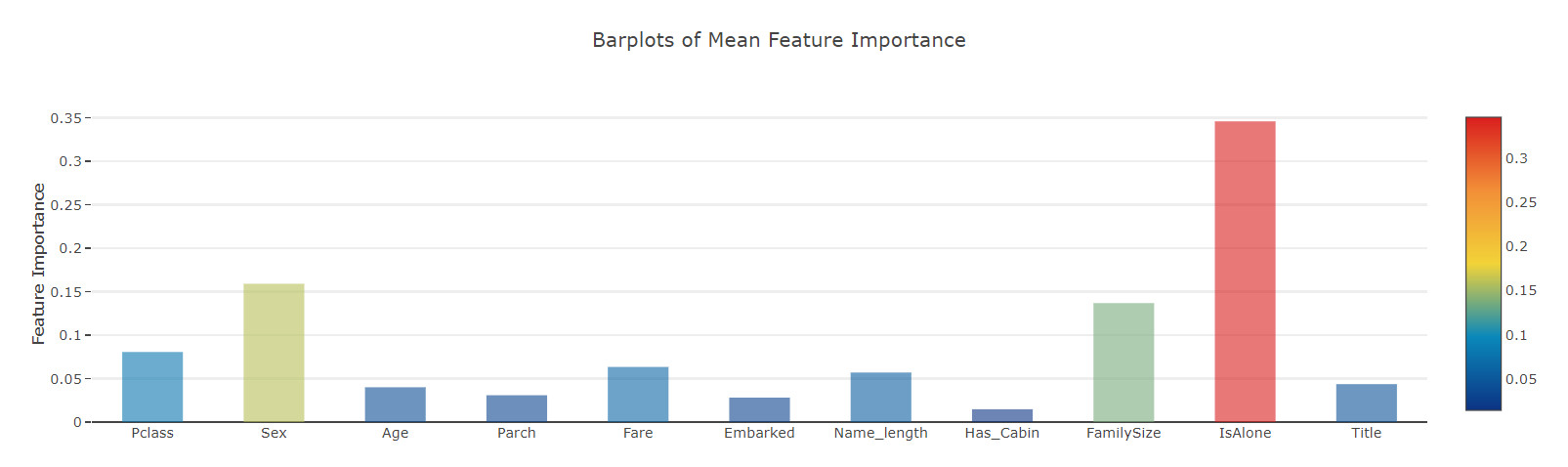
Now, let's calculate the average value of all feature importance and store it as a new column in the feature importance data box.
# mean value

feature_dataframe['mean'] = feature_dataframe.mean(axis= 1) # axis = 1 computes the mean row-wise
feature_dataframe.head(3)
Feature importance bar chart
y = feature_dataframe['mean'].values
x = feature_dataframe['features'].values
data = [go.Bar(
            x= x,
             y= y,
            width = 0.5,
            marker=dict(
               color = feature_dataframe['mean'].values,
            colorscale='Portland',
            showscale=True,
            reversescale = False
            ),
            opacity=0.6
        )]

layout= go.Layout(
    autosize= True,
    title= 'Barplots of Mean Feature Importance',
    hovermode= 'closest',
#     xaxis= dict(
#         title= 'Pop',
#         ticklen= 5,
#         zeroline= False,
#         gridwidth= 2,
#     ),
    yaxis=dict(
        title= 'Feature Importance',
        ticklen= 5,
        gridwidth= 2
    ),
    showlegend= False
)
fig = go.Figure(data=data, layout=layout)
py.iplot(fig, filename='bar-direct-labels')
Tier 2 forecast
First stage output as a new feature
Now that our first level prediction has been obtained, we can think that it essentially constructs a new set of features to be used as the training data of the next classifier. Therefore, according to the following code, our new column contains the first level prediction from the early classifier, and trains the next classifier on this basis.
base_predictions_train = pd.DataFrame( {'RandomForest': rf_oof_train.ravel(),
     'ExtraTrees': et_oof_train.ravel(),
     'AdaBoost': ada_oof_train.ravel(),
      'GradientBoost': gb_oof_train.ravel()
    })
base_predictions_train.head()
Correlation heat map
data = [
    go.Heatmap(
        z= base_predictions_train.astype(float).corr().values ,
        x=base_predictions_train.columns.values,
        y= base_predictions_train.columns.values,
          colorscale='Viridis',
            showscale=True,
            reversescale = True
    )
]
py.iplot(data, filename='labelled-heatmap')

x_train = np.concatenate(( et_oof_train, rf_oof_train, ada_oof_train, gb_oof_train, svc_oof_train), axis=1)
x_test = np.concatenate(( et_oof_test, rf_oof_test, ada_oof_test, gb_oof_test, svc_oof_test), axis=1)
Two level learning model based on XGBoost
Here, we choose the very famous boosted tree learning model library XGBoost. It is used to optimize the large-scale boosted tree algorithm.
gbm = xgb.XGBClassifier(
    #learning_rate = 0.02,
 n_estimators= 2000,
 max_depth= 4,
 min_child_weight= 2,
 #gamma=1,
 gamma=0.9,
 subsample=0.8,
 colsample_bytree=0.8,
 objective= 'binary:logistic',
 nthread= -1,
 scale_pos_weight=1).fit(x_train, y_train)
predictions = gbm.predict(x_test)
Generate submission file
# Generate Submission File
StackingSubmission = pd.DataFrame({ 'PassengerId': PassengerId,
                            'Survived': predictions })
StackingSubmission.to_csv("StackingSubmission.csv", index=False)
The level is limited. Please understand if there are some unexplainable places. If it is helpful to you, you are welcome to like the collection!