This series of articles is to explain Python OpenCV image processing knowledge. In the early stage, it mainly explains the introduction of image and the basic usage of OpenCV. In the middle stage, it explains various algorithms of image processing, including image sharpening operator, image enhancement technology, image segmentation, etc. in the later stage, it studies image recognition and image classification application in combination with in-depth learning. I hope the article is helpful to you. If there are deficiencies, please forgive me~
All source code of this series in github:
- https://github.com/eastmountyxz/ ImageProcessing-Python
The previous article introduced the basic knowledge of Python image processing. This article will explain the basic knowledge of OpenCV+Numpy image processing, including reading pixels and modifying pixels. The knowledge points are as follows:
- 1, Traditional pixel reading method
- 2, Traditional pixel modification method
- 3, Numpy pixel reading method
- 4, Numpy modify pixel method
- 5, Geometric drawing
1, Traditional pixel reading method
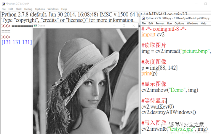
1. Grayscale image, return grayscale value Return value = image (position parameter), for example: P = img [88142] print (P)
# -*- coding:utf-8 -*-
import cv2

#Read picture
img = cv2.imread("picture.bmp", cv2.IMREAD_UNCHANGED)

#Gray image
p = img[88, 142]
print(p)

#Display image
cv2.imshow("Demo", img)

#Wait for display
cv2.waitKey(0)
cv2.destroyAllWindows()

#Write image
cv2.imwrite("testyxz.jpg", img)
The output results are as follows: [131]. Since the figure is a 24 bit BMP, B=G=R outputs three same results. If there is only one pixel in some images, a value is output.
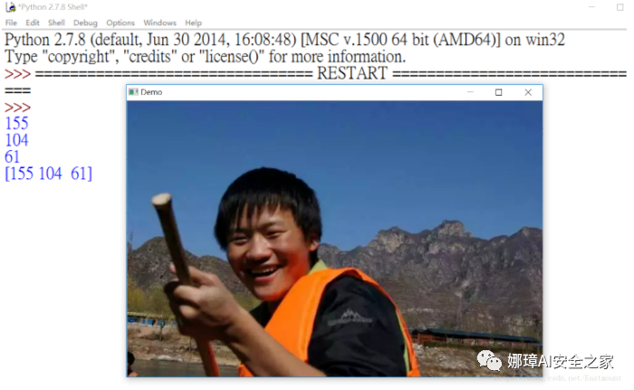
2.BGR image, the return values are B, G and R Example:
- b = img[78, 125, 0] print(b)
- g = img[78, 125, 1] print(g)
- r = img[78,125, 2] print(r)
# -*- coding:utf-8 -*-
import cv2

#Read picture
img = cv2.imread("test.jpg", cv2.IMREAD_UNCHANGED)

#BGR image
b = img[78, 125, 0]
print(b)
g = img[78, 125, 1]
print(g)
r = img[78, 125, 2]
print(r)

#Method 2
bgr = img[78, 125]
print(bgr)

#Display image
cv2.imshow("Demo", img)

#Wait for display
cv2.waitKey(0)
cv2.destroyAllWindows()

#Write image
cv2.imwrite("testyxz.jpg", img)
The output pixels and images are as follows:
- 155
- 104
- 61
- [155 104 61]
2, Traditional pixel modification method
1. Modify a single pixel value BGR image can directly access and modify pixel values through position parameters. The output results are as follows:
# -*- coding:utf-8 -*-
import cv2

#Read picture
img = cv2.imread("test.jpg", cv2.IMREAD_UNCHANGED)

#BGR image
print(img[78, 125, 0])
print(img[78, 125, 1])
print(img[78, 125, 2])

#Modify pixel
img[78, 125, 0] = 255
img[78, 125, 1] = 255
img[78, 125, 2] =255
print(img[78, 125])
img[78, 125] = [10, 10, 10]
print(img[78, 125, 0])
print(img[78, 125, 1])
print(img[78, 125, 2])

#Method 2
print(img[78, 125])
img[78, 125] = [10, 10, 10]
print(img[78, 125])
The output results are as follows. The pixel values of B, G and R are modified to 255 and 0 respectively by two methods.
- 155
- 104
- 61
- 255
- 255
- 255
- [255 255 255]
- [10 10 10]
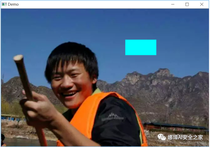
2. Modify area pixels
The region pixels are modified by accessing the position region of the image array. For example, [100:150400:500] accesses the region in rows 100 to 150 and columns 400 to 500, and then modifies the region pixels. The code is as follows:
# -*- coding:utf-8 -*-
import cv2

#Read picture
img = cv2.imread("test.jpg", cv2.IMREAD_UNCHANGED)

#BGR image
img[100:150, 400:500] = [255, 255, 0]

#Display image
cv2.imshow("Demo", img)

#Wait for display
cv2.waitKey(0)
cv2.destroyAllWindows()

#Write image
cv2.imwrite("testyxz.jpg", img)
The output result is as follows, [255, 255, 0] is light blue.
3, Numpy pixel reading method
Use Numpy to read pixels. The calling method is as follows:
- Return value = image. Item (position parameter)
# -*- coding:utf-8 -*-
import cv2
import numpy

#Read picture
img = cv2.imread("test.jpg", cv2.IMREAD_UNCHANGED)

#Numpy read pixel
blue = img.item(78, 100, 0)
green = img.item(78, 100, 1)
red = img.item(78, 100, 2)
print(blue)
print(green)
print(red)

#Display image
cv2.imshow("Demo", img)

#Wait for display
cv2.waitKey(0)
cv2.destroyAllWindows()
The output results are as follows. Note that the OpenCV read image channel is BGR, which can also be converted to RGB for processing.
- 155
- 104
- 61
4, Numpy modify pixel method
Use Numpy's itemset function to modify pixels. The call method is as follows:
- Image. Itemset (position, new value)
For example: img.itemset((88,99), 255)
# -*- coding:utf-8 -*-
import cv2
import numpy

#Read picture
img = cv2.imread("test.jpg", cv2.IMREAD_UNCHANGED)

#Numpy read pixel
print(img.item(78, 100, 0))
print(img.item(78, 100, 1))
print(img.item(78, 100, 2))
img.itemset((78, 100, 0), 100)
img.itemset((78, 100, 1), 100)
img.itemset((78, 100, 2), 100)
print(img.item(78, 100, 0))
print(img.item(78, 100, 1))
print(img.item(78, 100, 2))
The output results are as follows:
- 155
- 104
- 61
- 100
- 100
- 100
B, G and R can also be output at the same time. The core code is as follows:
print(img[78, 78])
img.itemset((78, 78, 0), 0)
img.itemset((78, 78, 1), 0)
img.itemset((78, 78, 2), 0)
print(img[78, 78])
#[155 104  61]
#[0 0 0]
5, Geometric drawing
This section mainly explains the drawing method of geometry in OpenCV, including:
- cv2.line()
- cv2.circle()
- cv2.rectangle()
- cv2.ellipse()
- cv2.polylines()
- cv2.putText()
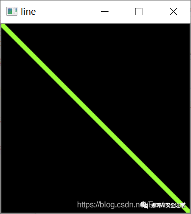
1. Draw a straight line
In OpenCV, to draw a straight line, you need to obtain the starting and ending coordinates of the straight line, and call cv2.line() function to realize this function. The prototype of this function is as follows:
- img = line(img, pt1, pt2, color[, thickness[, lineType[, shift]]]) – img represents the image to be drawn – pt1 represents the coordinates of the first point of the line segment – pt2 represents the coordinates of the second point of the line segment – color represents the line color, and an RGB tuple needs to be passed in. For example, (255,0,0) represents blue – thickness indicates the thickness of the line – lineType indicates the type of line – shift indicates the number of decimal places in the point coordinates
The following code is to draw a straight line, create a black image through np.zeros(), and then call cv2.line() to draw a straight line. The parameters include starting coordinates, color and thickness.
# -*- coding:utf-8 -*-
import cv2
import numpy as np

#Create black image
img = np.zeros((256,256,3), np.uint8)

#draw a straight line
cv2.line(img, (0,0), (255,255), (55,255,155), 5)

#Display image
cv2.imshow("line", img)

#Wait for display
cv2.waitKey(0)
cv2.destroyAllWindows()
The output result is as shown in the figure. Draw a straight line from coordinates (0,0) to (255255). The color of the straight line is (55255155) and the thickness is 5.
After mastering the basic line drawing method, we can make simple changes. For example, the following code adds a simple loop to draw the graph into four parts.
# -*- coding:utf-8 -*-
import cv2
import numpy as np

#Create black image
img = np.zeros((256,256,3), np.uint8)

#draw a straight line
i = 0
while i<255:
    cv2.line(img, (0,i), (255,255-i), (55,255,155), 5)
    i = i + 1

#Display image
cv2.imshow("line", img)

#Wait for display
cv2.waitKey(0)
cv2.destroyAllWindows()
The output results are shown in the figure.

2. Draw rectangle
In OpenCV, rectangle drawing is realized by cv2.rectangle() function. The prototype of this function is as follows:
- img = rectangle(img, pt1, pt2, color[, thickness[, lineType[, shift]]]) – img represents the image to be drawn – pt1 represents the position coordinates of the upper left corner of the rectangle – pt2 represents the position coordinates of the lower right corner of the rectangle – color indicates the color of the rectangle – thickness indicates the thickness of the border – lineType indicates the type of line – shift indicates the number of decimal places in the point coordinates
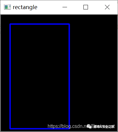
The following code is to draw a rectangle, create a black image through np.zeros(), and then call cv2.rectangle() to draw the rectangle.
# -*- coding:utf-8 -*-
import cv2
import numpy as np

#Create black image
img = np.zeros((256,256,3), np.uint8)

#draw rectangle
cv2.rectangle(img, (20,20), (150,250), (255,0,0), 2)

#Display image
cv2.imshow("rectangle", img)

#Wait for display
cv2.waitKey(0)
cv2.destroyAllWindows()
The output results are shown in the figure. The coordinates from the upper left corner are (20,20) and the coordinates from the lower right corner are (150250). The color of the drawn rectangle is blue (255,0,0) and the thickness is 2.
3. Draw a circle
In OpenCV, rectangle drawing is realized by cv2.rectangle() function. The prototype of this function is as follows:
- img = circle(img, center, radius, color[, thickness[, lineType[, shift]]]) – img indicates the image of the circle to be drawn – Center represents the coordinates of the center of the circle – radius indicates the radius of the circle – color indicates the color of the circle – thickness if it is positive, it indicates the thickness of the circular contour; A negative thickness indicates that a filled circle is to be drawn – lineType indicates the boundary type of the circle – shift indicates the number of decimal places in the center coordinate and radius value
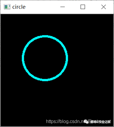
The following code is to draw a circle.
# -*- coding:utf-8 -*-
import cv2
import numpy as np

#Create black image
img = np.zeros((256,256,3), np.uint8)

#Draw circle
cv2.circle(img, (100,100), 50, (255,255,0), -1)

#Display image
cv2.imshow("circle", img)

#Wait for display
cv2.waitKey(0)
cv2.destroyAllWindows()
The output result is shown in the figure. It draws a circle with radius of 50, color of (255255,0) and thickness of 4 at the position where the circle is (100100).
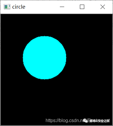
Note that if the thickness is set to "- 1", the drawn circle is solid, as shown in the figure.
- cv2.circle(img, (100,100), 50, (255,255,0), -1)
4. Draw ellipse
In OpenCV, drawing an ellipse is complex. You need to input several more parameters, such as the position coordinates of the center point, the length of the major axis and minor axis, the rotation angle of the ellipse in the counterclockwise direction, etc. The prototype of cv2.ellipse() function is as follows:
- img = ellipse(img, center, axes, angle, startAngle, endAngle, color[, thickness[, lineType[, shift]]]) – img represents the image that needs to draw an ellipse – Center represents the center coordinates of the ellipse – axes indicates the length of the shaft (short radius and long radius) – angle indicates the angle of deflection (counterclockwise rotation) – startAngle represents the angle of the starting angle of the arc (counterclockwise rotation) – endAngle represents the angle of the end angle of the arc (counterclockwise rotation) – color indicates the color of the line – thickness, if positive, indicates the thickness of the elliptical contour; A negative value indicates that you want to draw a fill ellipse – lineType indicates the boundary type of the circle – shift indicates the number of decimal places in the center coordinate and axis value
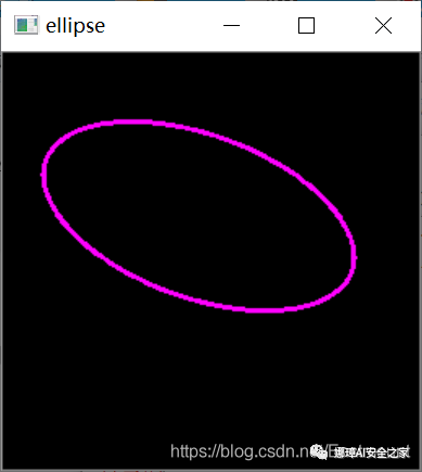
The following is the code for drawing an ellipse.
# -*- coding:utf-8 -*-
import cv2
import numpy as np

#Create black image
img = np.zeros((256,256,3), np.uint8)

#Draw ellipse
#The major axis and minor axis of the ellipse center (120100) are (100,50)
#The deflection angle is 20
#Angle of arc start angle 0 angle of arc end angle 360
#Color (255,0255) line thickness 2
cv2.ellipse(img, (120, 100), (100, 50), 20, 0, 360, (255, 0, 255), 2)

#Display image
cv2.imshow("ellipse", img)

#Wait for display
cv2.waitKey(0)
cv2.destroyAllWindows()
The output result is shown in the figure. The ellipse center is (120100), the long axis is 100, the short axis is 50, the deflection angle is 20, the angle of the arc starting angle is 0, and the angle of the arc ending angle is 360, indicating a complete ellipse. The color drawn is (255,0255) and the thickness is 2.
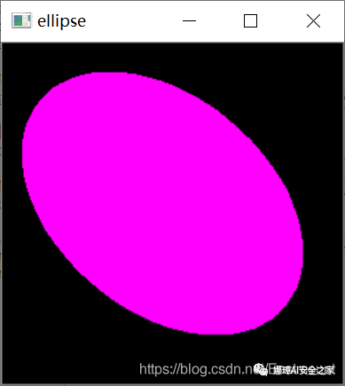
The following code is to draw a solid ellipse.
# -*- coding:utf-8 -*-
import cv2
import numpy as np

#Create black image
img = np.zeros((256,256,3), np.uint8)

#Draw ellipse
cv2.ellipse(img, (120, 120), (120, 80), 40, 0, 360, (255, 0, 255), -1)

#Display image
cv2.imshow("ellipse", img)

#Wait for display
cv2.waitKey(0)
cv2.destroyAllWindows()
Draw the graph as shown in the figure.
5. Draw polygon
In OpenCV, the cv2.polylines() function is used to draw polygons. It needs to specify the coordinates of each vertex and construct polygons through these points. The prototype of the function is as follows:
- img = polylines(img, pts, isClosed, color[, thickness[, lineType[, shift]]]) – img represents the image to be drawn – center represents a polygon curve array – isClosed indicates whether the drawn polygon is closed, and False indicates not closed – color indicates the color of the line – thickness indicates the thickness of the line – lineType indicates the boundary type – shift indicates the number of decimal places in vertex coordinates
The following is the code for drawing a polygon.
# -*- coding:utf-8 -*-
import cv2
import numpy as np
#Create black image
img = np.zeros((256,256,3), np.uint8)
#draw a polygon
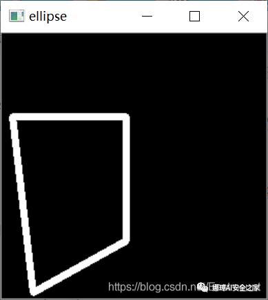
pts = np.array([[10,80], [120,80], [120,200], [30,250]])
cv2.polylines(img, [pts], True, (255, 255, 255), 5)
#Display image
cv2.imshow("ellipse", img)
#Wait for display
cv2.waitKey(0)
cv2.destroyAllWindows()
The output result is as shown in the figure, and the drawn polygon is a white closed figure.
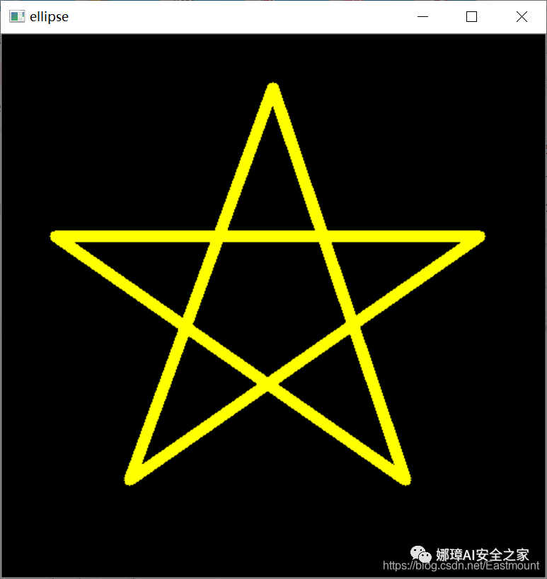
The following code is to draw a pentagram polygon.
# -*- coding:utf-8 -*-
import cv2
import numpy as np

#Create black image
img = np.zeros((512,512,3), np.uint8)

#draw a polygon
pts = np.array([[50, 190], [380, 420], [255, 50], [120, 420], [450, 190]])
cv2.polylines(img, [pts], True, (0, 255, 255), 10)

#Display image
cv2.imshow("ellipse", img)

#Wait for display
cv2.waitKey(0)
cv2.destroyAllWindows()
The output result is shown in the figure. It connects the left of the five vertices to form a yellow pentagram.
6. Draw text
In OpenCV, call the cv2.putText() function to add the corresponding text, its function prototype is as follows:
- img = putText(img, text, org, fontFace, fontScale, color[, thickness[, lineType[, bottomLeftOrigin]]]) – img represents the image to be drawn – text indicates the text to be drawn – org indicates the position to be drawn, and the image is in the lower left corner of the Chinese text string – fontFace indicates the font type. see cv::HersheyFonts for details – fontScale represents the size of the font and is calculated as a scale factor multiplied by the font specific base size – color indicates the color of the font – thickness indicates the thickness of the font – lineType indicates the boundary type – bottomLeftOrigin if true, the image data origin is in the lower left corner, otherwise it is in the upper left corner
The following is the code for drawing text.
# -*- coding:utf-8 -*-
import cv2
import numpy as np
#Create black image
img = np.zeros((256,256,3), np.uint8)
#Draw text
font = cv2.FONT_HERSHEY_SIMPLEX
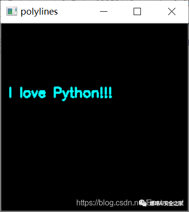
cv2.putText(img, 'I love Python!!!',
(10, 100), font, 0.6, (255, 255, 0), 2)
#Display image
cv2.imshow("polylines", img)
#Wait for display
cv2.waitKey(0)
cv2.destroyAllWindows()
The output result is as shown in the figure, and the drawn text is "I love Python!!!".
4, Summary
This is the end of this basic article. I hope the article will be helpful to you. If there are mistakes or deficiencies, please forgive me. This article starts with CSDN column, so as to help more students, update the official account number and cheer up!
- 1, Traditional pixel reading method
- 2, Traditional pixel modification method
- 3, Numpy pixel reading method
- 4, Numpy modify pixel method
- 5, Geometric drawing
reference:
- [1] Luo Zijiang. Image processing in Python [M]. Science Press, 2020
- [2] https://blog.csdn.net/eastmount/category_9278090.html
- [3] Gonzalez. Digital image processing (3rd Edition) [M]. Electronic Industry Press, 2013
- [4] Ruan Qiuqi. Digital image processing (3rd Edition) [M]. Electronic Industry Press, 2008
- [5] Mao Xingyun, Leng Xuefei. Introduction to OpenCV3 programming [M]. Electronic Industry Press, 2015
- [6] Zhang Zheng. Digital image processing and machine vision -- implementation with Visual C + + and Matlab
- [6] Netease cloud classroom_ Gordon education. Python+OpenCV image processing