0. Preface
Some powerful models have been used before, such as VGG16 in the field of image classification, YoloV5 in the field of target detection, Yolact in the field of instance segmentation, etc. But only after the environment is configured for training, the interface of the source code can be modified slightly to meet their own needs. PyTorch has never been used to build and train a model from scratch.
Just recently, I'm learning PyTorch systematically. I'll summarize how to build and train a neural network model from scratch.
1. Use torchvision to load the dataset and perform preprocessing
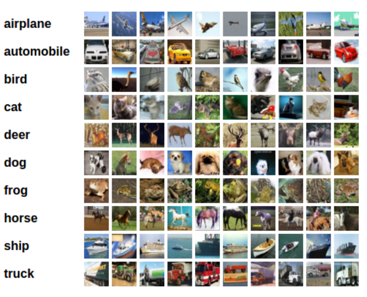
The dataset we use is CIFAR10, which has 10 categories and the image size is 3 x 32 x 32, as shown below:
The code is as follows, and there are notes in the code in important places
import torch
import cv2
import numpy as np
from torchvision import datasets, transforms
import torchvision

# 1. Use torchvision to load the dataset and perform preprocessing
transform = transforms.Compose([transforms.ToTensor(),  # Convert image to tensor
                                transforms.Normalize((0.5,0.5,0.5), (0.5,0.5,0.5)),  # Normalization processing
                              ])
# Load training and test sets
trainset = torchvision.datasets.CIFAR10(root='E:\\Machine Learning\\PyTorch\\CIFAR10', train=True, download=True, transform=transform)
trainloader = torch.utils.data.DataLoader(trainset, batch_size=4, shuffle=True, num_workers=2)
testset = torchvision.datasets.CIFAR10(root='E:\\Machine Learning\\PyTorch\\CIFAR10', train=False, download=True, transform=transform)
testloader = torch.utils.data.DataLoader(testset, batch_size=4, shuffle=False, num_workers=2)
2. Define (build) your own neural network
The code and notes are as follows. The whole structure is very simple, that is, two volume layers, two maximum pool layers, and finally connect three full connection layers.
# 2. Define convolutional neural network
import torch.nn as nn
import torch.nn.functional as F

class MyModel(nn.Module):  #  Inherit nn.Module
    # Define network structure
    def __init__(self):
        super(MyModel, self).__init__()
        self.conv1 = nn.Conv2d(3,6,5)
        self.pool = nn.MaxPool2d(2,2)
        self.conv2 = nn.Conv2d(6,16,5)
        self.fc1 = nn.Linear(16*5*5, 120)
        self.fc2 = nn.Linear(120, 84)
        self.fc3 = nn.Linear(84, 10)
    # Define forward propagation process
    def forward(self, x):
        x = self.pool(F.relu(self.conv1(x)))
        x = self.pool(F.relu(self.conv2(x)))
        x = x.view(-1, 16*5*5)
        x = F.relu(self.fc1(x))
        x = F.relu(self.fc2(x))
        x = self.fc3(x)

        return x

Net = MyModel()
3. Define Loss Function and Optimizer
The back propagation of neural network requires a loss function. Because it is a multi classification problem, we use the cross entropy loss function:
# 3. Define loss function and optimizer
import torch.optim as optim

criterion = nn.CrossEntropyLoss()  # Multi classification problem, using cross entropy loss function
optimizer = optim.SGD(Net.parameters(), lr=0.001, momentum=0.9)  # Using SGD optimizer
4. Training neural network
Then we began to train our model, training 2 epoch and batch in total_ Size = 4, first train with CPU and see how the time is.
# 4. Training neural network
epochs = 2  # Train two epoch, batch_ Size = 4 (the size of batch_size is defined in torch.utils.data.DataLoader in the first step)
e1 = cv2.getTickCount()  # Record training time
for epoch in range(epochs):
    total_loss = 0.0
    for i, data in enumerate(trainloader, 0):
        # Get inputs
        inputs, labels = data
        optimizer.zero_grad()
        # forward + backward + optimize
        # Forward propagation + back propagation + update parameters
        outputs = Net(inputs)  # Forward propagation to obtain outputs
        loss = criterion(outputs, labels)  # The loss function is obtained
        loss.backward()  # Backward propagation
        optimizer.step()  # Update parameters

        # Output training process
        total_loss += loss.item()
        if (i+1) % 1000 == 0:  # loss is output every 1000 times (4000 images)
            print('The first{}individual epoch: The first{:5d}Times: current training loss loss Is:{:.3f}'.format(epoch+1, i+1, total_loss/1000))
            total_loss = 0.0

e2 = cv2.getTickCount()
print('use CPU Total training time:{} s'.format((e2-e1)/cv2.getTickFrequency()))
# Output results:
1st epoch: 1000th time: current training loss loss Is: 2.294
 1st epoch: 2000: current training loss loss Is: 2.087
 1st epoch: 3000: current training loss loss Is: 1.902
 1st epoch: 4000: current training loss loss Is: 1.799
 1st epoch: Session 5000: current training loss loss Is: 1.709
 1st epoch: 6000: current training loss loss Is: 1.660
 1st epoch: 7000: current training loss loss Is: 1.623
 1st epoch: 8000: current training loss loss Is: 1.586
 1st epoch: 9000: current training loss loss Is: 1.550
 1st epoch: 10000 times: current training loss loss Is: 1.497
 1st epoch: 11000: current training loss loss Is: 1.468
 1st epoch: 12000 times: current training loss loss Is: 1.469
 2nd epoch: 1000th time: current training loss loss Is: 1.392
 2nd epoch: 2000: current training loss loss Is: 1.382
 2nd epoch: 3000: current training loss loss Is: 1.364
 2nd epoch: 4000: current training loss loss Is: 1.361
 2nd epoch: Session 5000: current training loss loss Is: 1.344
 2nd epoch: 6000: current training loss loss Is: 1.349
 2nd epoch: 7000: current training loss loss Is: 1.313
 2nd epoch: 8000: current training loss loss Is: 1.327
 2nd epoch: 9000: current training loss loss Is: 1.306
 2nd epoch: 10000 times: current training loss loss Is: 1.302
 2nd epoch: 11000: current training loss loss Is: 1.275
 2nd epoch: 12000 times: current training loss loss Is: 1.288
 use CPU Total training time: 83.7945317 s
It took 83.79 seconds.
5. Test model results
# 5. How accurate is the test model

correct = 0
total = 0

e1 = cv2.getTickCount()  # Record the test time
with torch.no_grad():  # Do not track gradient
    for data in testloader:
        images, labels = data
        outputs = Net(images)
        _, predicted = torch.max(outputs.data, 1)
        total += labels.size(0)
        correct += (predicted == labels).sum().item()

e2 = cv2.getTickCount()
print('use CPU Total test time:{} s'.format((e2-e1)/cv2.getTickFrequency()))
print('The accuracy on the test set is:{:.3f}%'.format(correct*100/total))
Let's see what happens
# result
 use CPU Total test time: 5.3146039 s
 The accuracy on the test set is: 55.460%
The accuracy rate is about 55%. Although it is not high, it can be seen that our model has indeed learned something (because the accuracy rate of random prediction for 10 classification problems is about 10%). And the purpose of this blog is to sort out the general process of training neural networks, rather than to build an excellent model.
6. Too slow CPU? Change GPU training and try!
First, check whether the corresponding versions of cuda and cudnn are installed. The specific installation steps will not be mentioned. There are many excellent tutorials on csdn.
# Check whether the corresponding version of cuda is installed on the computer
device = torch.device('cuda:0' if torch.cuda.is_available else 'cpu')
print('Equipment name: ', device)
print('see cuda edition: ', torch.version.cuda)
# result
 Equipment name:  cuda:0
 see cuda Version: 10.1
PyTorch is very convenient to use GPU for training. Compared with CPU training in step 4, it only needs to add two lines of code:
(1) Load the neural network model into cuda
(2) Load data into cuda
The codes and notes are as follows:
# 6. Training neural network with GPU
######  The first is different   ########
Net.to(device)  # Load the neural network model into cuda
epochs = 2  # Train two epoch, batch_ Size = 4 (the size of batch_size is defined in torch.utils.data.DataLoader in the first step)
e1 = cv2.getTickCount()  # Record training time
for epoch in range(epochs):
    total_loss = 0.0
    for i, data in enumerate(trainloader, 0):
        # Get inputs
        inputs, labels = data
        ######  The second is different   ########
        inputs, labels = inputs.to(device), labels.to(device)  # Load data into cuda
        optimizer.zero_grad()
        # forward + backward + optimize
        # Forward propagation + back propagation + update parameters
        outputs = Net(inputs)  # Forward propagation to obtain outputs
        loss = criterion(outputs, labels)  # The loss function is obtained
        loss.backward()  # Backward propagation
        optimizer.step()  # Update parameters

        # Output training process
        total_loss += loss.item()
        if (i+1) % 1000 == 0:  # loss is output every 1000 times (4000 images)
            print('The first{}individual epoch: The first{:5d}Times: current training loss loss Is:{:.3f}'.format(epoch+1, i+1, total_loss/1000))
            total_loss = 0.0

e2 = cv2.getTickCount()
print('use CPU Total training time:{} s'.format((e2-e1)/cv2.getTickFrequency()))
See what happens:
# result
 1st epoch: 1000th time: current training loss loss Is: 2.231
 1st epoch: 2000: current training loss loss Is: 2.032
 1st epoch: 3000: current training loss loss Is: 1.872
 1st epoch: 4000: current training loss loss Is: 1.745
 1st epoch: Session 5000: current training loss loss Is: 1.702
 1st epoch: 6000: current training loss loss Is: 1.634
 1st epoch: 7000: current training loss loss Is: 1.603
 1st epoch: 8000: current training loss loss Is: 1.548
 1st epoch: 9000: current training loss loss Is: 1.513
 1st epoch: 10000 times: current training loss loss Is: 1.494
 1st epoch: 11000: current training loss loss Is: 1.459
 1st epoch: 12000 times: current training loss loss Is: 1.452
 2nd epoch: 1000th time: current training loss loss Is: 1.396
 2nd epoch: 2000: current training loss loss Is: 1.372
 2nd epoch: 3000: current training loss loss Is: 1.350
 2nd epoch: 4000: current training loss loss Is: 1.361
 2nd epoch: Session 5000: current training loss loss Is: 1.338
 2nd epoch: 6000: current training loss loss Is: 1.312
 2nd epoch: 7000: current training loss loss Is: 1.322
 2nd epoch: 8000: current training loss loss Is: 1.289
 2nd epoch: 9000: current training loss loss Is: 1.277
 2nd epoch: 10000 times: current training loss loss Is: 1.269
 2nd epoch: 11000: current training loss loss Is: 1.293
 2nd epoch: 12000 times: current training loss loss Is: 1.283
 use CPU Total training time: 74.0288839 s
Compared with 83 seconds of CPU, the GPU takes 74 seconds, which is faster, but the improvement is not obvious enough. This is because our network is very small and has few parameters. In addition, the GPU of my notebook is also very old, 1050 core display.
We are trying to infer how much acceleration will be achieved by using GPU:
# 6. Use GPU to infer

correct = 0
total = 0
Net.to(device)  # Load the neural network model into cuda

e1 = cv2.getTickCount()  # Record the test time
with torch.no_grad():  # Do not track gradient
    for data in testloader:
        images, labels = data
        images, labels = images.to(device), labels.to(device) # Load data into cuda
        outputs = Net(images)
        _, predicted = torch.max(outputs.data, 1)
        total += labels.size(0)
        correct += (predicted == labels).sum().item()

e2 = cv2.getTickCount()
print('use CPU Total test time:{} s'.format((e2-e1)/cv2.getTickFrequency()))
print('The accuracy on the test set is:{:.3f}%'.format(correct*100/total))
See what happens
# result
 use CPU Total test time: 4.3125164 s
 The accuracy on the test set is 54.090%
Compared with 5.3 seconds for CPU inference and 4.3 seconds for GPU inference, the speed is also improved.