Previously, we have successfully completed the reproduction of the first 20 key charts of CNS chart reproduction album. Now we start the second wave of chart reproduction and will touch a lot of supplementary charts. Table of contents and previous code summary The second wave of CNS chart reproduction album opens .
If you only see this series now, you are recommended to read the article of CELL magazine: therapy induced evolution of human lung cancer reviewed by single CELL RNA sequencing, because the author provides a complete set of codes in: https://github.com/czbiohub/scell_lung_adenocarcinoma, the researchers collected 49 biopsies (biopsy) from 30 patients, which were divided into three types: before treatment (TKI naive [TN]), after targeted treatment, tumor regression or stable (RD), and after targeted treatment, tumor still growth (PD, up subsequence progressive disease), so that the single-CELL transcriptome data are very rich!
stay The second wave of CNS chart reproduction album opens We can see the previous dimensionality reduction clustering, but we don't know why lymphocytes and myeloid lines such as T and B are slightly mixed, and they are not completely different from epithelial cells in umap.
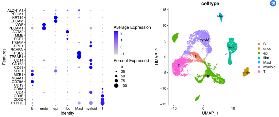
Is it because I didn't integrate samples or patients? I face in front of you The second wave of CNS chart reproduction album opens It is pointed out in the tutorial that CCA integration is not necessary for single cells of smart-seq2 technology, mainly because each sample actually has hundreds of cells, not thousands of cells for each sample of 10X technology.
We preliminarily reduce the dimension of a tumor single-cell transcriptome data, cluster and cluster it, and each single-cell subgroup is saved independently as a seurat object. Next, it is easy to extract the expression matrix in T and B lymphocyte objects as a normal diploid reference cell to deduce the tumor copy number from the single-cell transcriptome data, Then the tumor copy number was inferred from the epithelial cell expression matrix!
rm(list=ls())
library(Seurat)
library(ggplot2)
library(clustree)
library(cowplot)
library(dplyr)
sce.all=readRDS( "2-int/sce.all_int.rds")
sce.all
table(sce.all@meta.data$seurat_clusters)
load(file = '3-cell/phe_by_markers.Rdata')
table(phe$celltype)

sce.all$celltype=phe$celltype
sce.all.list <- SplitObject(sce.all , split.by = "celltype")
sce.all.list

for (i in names(sce.all.list)) {
  epi_mat = sce.all.list[[i]]@assays$RNA@counts
  epi_phe = sce.all.list[[i]]@meta.data
  sce=CreateSeuratObject(counts = epi_mat,
                         meta.data = epi_phe )
  sce
  table(sce@meta.data$orig.ident)
  save(sce,file = paste0(i,'.Rdata'))
}
The obtained documents are as follows;
   21M  8 19 16:46 B.Rdata
  9.2M  8 19 16:46 Mast.Rdata
   61M  8 19 16:46 T.Rdata
   18M  8 19 16:46 endo.Rdata
  161M  8 19 16:46 epi.Rdata
   58M  8 19 16:46 fibo.Rdata
  101M  8 19 16:45 myeloid.Rdata
In addition, please don't ask me for these Rdata files, but after you read the previous ones The second wave of CNS chart reproduction album opens Tutorial, these code run on their own to produce all the data files!
In fact, we are in the tutorial: CNS chart reproduction 09 - epithelial cells can be distinguished as malignant or not It is mentioned that only about 3700 of more than 5000 epithelial cells are malignant cells, but the technical differences between copykat and inforcnv in inferring tumor copy number variation from single-cell transcriptome data have not been explored.
Input data needed to build both algorithms
Inforcnv algorithm needs three files, but copykat only needs one file. We make it together here.
rm(list=ls())
options(stringsAsFactors = F)
library(Seurat)
load(file = 'first_sce.Rdata')  # It's just epithelial cells
epiMat=as.data.frame(GetAssayData( sce , slot='counts',assay='RNA'))
load('../Rdata-celltype/B.Rdata') # It's just B lymphocytes
B_cellMat=as.data.frame(GetAssayData( sce, slot='counts',assay='RNA'))
load('../Rdata-celltype/T.Rdata') # It's just T lymphocytes
T_cellsMat=as.data.frame(GetAssayData( sce, slot='counts',assay='RNA'))

B_cellMat=B_cellMat[,sample(1:ncol(B_cellMat),800)]
T_cellsMat=T_cellsMat[,sample(1:ncol(T_cellsMat),800)]
dat=cbind(epiMat,B_cellMat,T_cellsMat)

groupinfo=data.frame(v1=colnames(dat),
                     v2=c(rep('epi',ncol(epiMat)),
                          rep('spike-B_cell',300),
                          rep('ref-B_cell',500),
                          rep('spike-T_cells',300),
                          rep('ref-T_cells',500)))

library(AnnoProbe)
geneInfor=annoGene(rownames(dat),"SYMBOL",'human')
colnames(geneInfor)
geneInfor=geneInfor[with(geneInfor, order(chr, start)),c(1,4:6)]
geneInfor=geneInfor[!duplicated(geneInfor[,1]),]
length(unique(geneInfor[,1]))
head(geneInfor)
## Sex chromosomes can be removed here
# You can also change the way chromosomes are sorted
dat=dat[rownames(dat) %in% geneInfor[,1],]
dat=dat[match( geneInfor[,1], rownames(dat) ),]
dim(dat)
expFile='expFile.txt'
write.table(dat,file = expFile,sep = '\t',quote = F)
groupFiles='groupFiles.txt'
head(groupinfo)
write.table(groupinfo,file = groupFiles,sep = '\t',quote = F,col.names = F,row.names = F)
head(geneInfor)
geneFile='geneFile.txt'
write.table(geneInfor,file = geneFile,sep = '\t',quote = F,col.names = F,row.names = F)
First, follow the inforcnv process
With the previous three files, the inforcnv process is super simple! The real core code is the inforcnv:: run function, which comes from the inforcnv package!
The code is as follows:
options(stringsAsFactors = F)
library(Seurat)
library(gplots)
library(ggplot2)

expFile='expFile.txt'
groupFiles='groupFiles.txt'
geneFile='geneFile.txt'

library(infercnv)
infercnv_obj = CreateInfercnvObject(raw_counts_matrix=expFile,
                                    annotations_file=groupFiles,
                                    delim="\t",
                                    gene_order_file= geneFile,
                                    ref_group_names=c("ref-B_cell",'ref-T_cells'))  ## This depends on the information in your grouping information


# cutoff=1 works well for Smart-seq2, and cutoff=0.1 works well for 10x Genomics
infercnv_obj2 = infercnv::run(infercnv_obj,
                              cutoff=0.1, # cutoff=1 works well for Smart-seq2, and cutoff=0.1 works well for 10x Genomics
                              out_dir= "infercnv_output",  # dir is auto-created for storing outputs
                              cluster_by_groups=F,   # cluster
                              hclust_method="ward.D2", plot_steps=F)
The results are as follows:
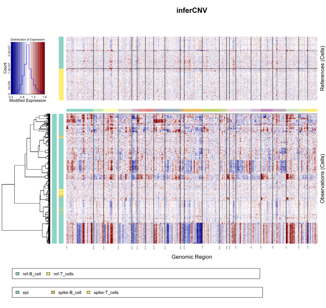
infercnv
It is easy to see that the normal cells we specially added are indeed determined as normal cells. At the same time, about one-third of epithelial cells will also be determined as normal cells. Follow the previous tutorial: CNS chart reproduction 09 - epithelial cells can be distinguished as malignant or not Mentioned that of the more than 5000 epithelial cells, only about 3700 are malignant cells, which is consistent.
Then go through the copykat process
With the previous three files, the copykat process is super simple! The real core code is the copykat function, which comes from the copykat package!
The code is as follows:
options(stringsAsFactors = F)
library(Seurat)
library(gplots)
library(ggplot2)

expFile='expFile.txt'
groupFiles='groupFiles.txt'
geneFile='geneFile.txt'

library(copykat)
exp.File <- read.delim( expFile , row.names=1)
exp.File[1:4,1:4]
groupFiles <- read.delim( groupFiles , header=FALSE)
head(groupFiles)

head( colnames(exp.File))
colnames(exp.File)=gsub('^X','', colnames(exp.File))
colnames(exp.File)=gsub('[.]','-', colnames(exp.File))
head( colnames(exp.File))

table(groupFiles$V2)
normalCells <-  colnames(exp.File)[grepl("ref",groupFiles$V2)]
head(normalCells)
Sys.time()
res <- copykat(rawmat=exp.File,  # Prepared expression matrix
                           id.type="S", # Choose symbol because it is in our expression matrix
                           ngene.chr=5,
                           win.size=25,
                           KS.cut=0.1,
                           sam.name="test",  # Prefix of a series of output files
                           distance="euclidean",
                           norm.cell.names=normalCells, # Name of normal cell
                           n.cores=1,
                           output.seg="FLASE")
Sys.time()
save(res,file = 'ref-of-copykat.Rdata')
You can see:
> Sys.time()
[1] "2021-12-02 10:14:49 CST"
# The operation process of the copykat function will also record the time itself
[1] "running copykat v1.0.5 updated 07/15/2021"
[1] "step1: read and filter data ..."
[1] "22493 genes, 6830 cells in raw data"
[1] "12355 genes past LOW.DR filtering"
[1] "step 2: annotations gene coordinates ..."
[1] "start annotation ..."
[1] "step 3: smoothing data with dlm ..."
[1] "step 4: measuring baselines ..."
[1] "896 known normal cells found in dataset"
[1] "run with known normal..."
[1] "baseline is from known input"
[1] "step 5: segmentation..."
[1] "step 6: convert to genomic bins..."
[1] "step 7: adjust baseline ..."
[1] "step 8: final prediction ..."
[1] "step 9: saving results..."
[1] "step 10: ploting heatmap ..."
Time difference of 4.091698 hours
> Sys.time()
[1] "2021-12-02 14:20:19 CST"
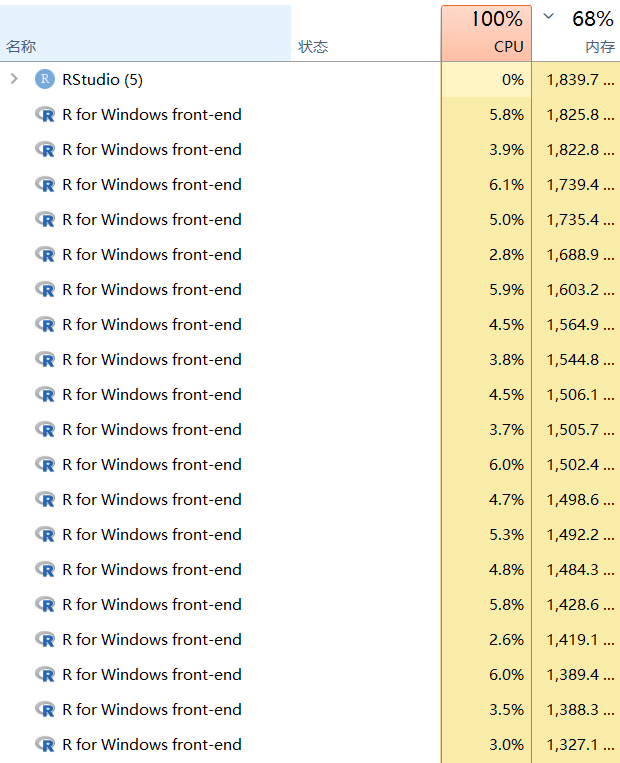
You can see that less than 7000 cells still need to run for 4 hours, but you can speed up this progress by setting the number of threads! Unfortunately, this function is not supported on Windows system platform:
Error in parallel::mclapply(1:ncol(norm.mat), dlm.sm, mc.cores = n.cores) :
  'mc.cores' > 1 is not supported on Windows
However, if you can also save the country by splitting the samples and then paralleling all the samples, it is also regarded as parallel computing:
ls -d S*|while read id;do
echo $id;
cd $id;
nohup Rscript.exe ../scripts/step4-run-copykat.R &
cd ../
done
For example, you store a matrix with the file name expFile.txt in each sample folder (folder beginning with S)
Any user can make a script: step4-run-copykat.R for parallelism as shown above.
Windows parallelism
In this way, each patient can run for more than ten minutes, super fast!
Then let's take a look at the results of copykat in the mixed group of all patients!
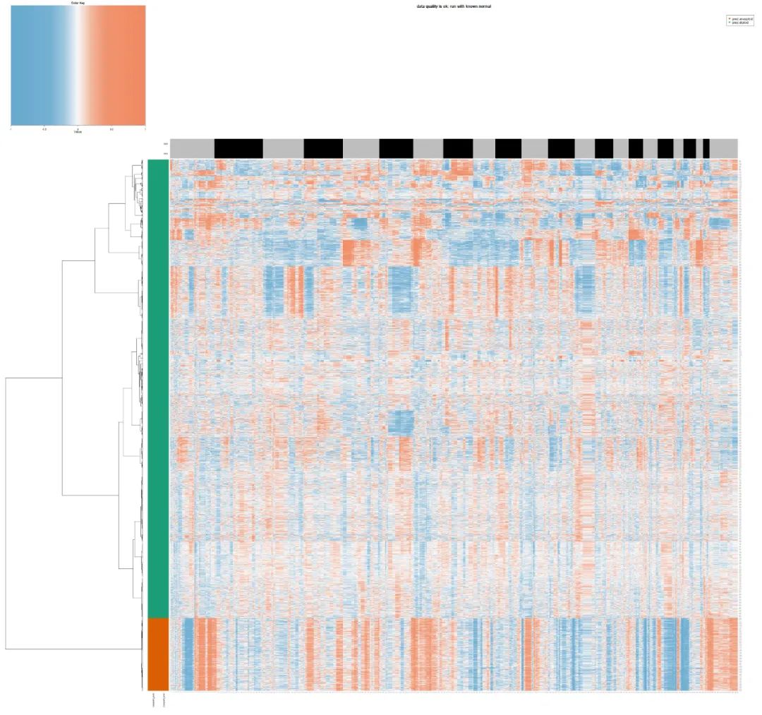
test_copykat_heatmap
It is amazing that this algorithm is a little loose in judging the malignancy of epithelial cells. A large number of aneuploid malignant cells we see with the naked eye are actually missed by the algorithm. There are less than 1000 cells defined as malignant epithelial cells by this algorithm:
               aneuploid diploid
  epi                 851    3965
  ref-B_cell            1     411
  ref-T_cells           0     480
  spike-B_cell          1     228
  spike-T_cells         0     288
It's really strange, because a lot of other cells look malignant to our naked eyes. They should be aneuploid. I don't know why they are wrongly judged as diploid by this algorithm. Maybe our data set is smart-seq2, not a common 10x data set?