Handwritten Number Recognition, Machine Learning "Classification" Learning Notes - From Geron's "Machine Learning Practice"
"hello word" in the field of image recognition
MNIST
Get MNIST code, 70,000 handwritten digital pictures - - 28x28 pixels 0-255 black and white pixels
Scitkit-Learn loaded datasets are usually dictionary structures
(The dataset needs to be downloaded here. It takes a long time. data_home saves the path so that you can't find the data there if you set the path in advance.)
from sklearn.datasets import fetch_openml
mnist = fetch_openml('mnist_784',version=1,data_home='./datasets',as_frame=False)
mnist.keys()
dict_keys(['data', 'target', 'frame', 'categories', 'feature_names', 'target_names', 'DESCR', 'details', 'url'])
Note: here mnist = fetch_openml('mnist_784', version=1,data_home='. /datasets', as_frame=False) There is no as_frame=False in the book, and when there is no such sentence, the data cannot be read after it
To see what the code on git-hub says
Warning: since Scikit-Learn 0.24, fetch_openml() returns a Pandas DataFrame by default. To avoid this and keep the same code as in the book, we use as_frame=False.
Visible is the difference between the data format and the version update
X,y = mnist["data"],mnist["target"]
X.shape
(70000, 784)
y.shape
(70000,)
Show pictures using imgshow() in Matplotlib
import matplotlib as mpl
import matplotlib.pyplot as plt
some_digit = X[0]
some_digit_image = some_digit.reshape(28,28)

plt.imshow(some_digit_image,cmap="binary")
plt.axis("off")
plt.show()

y[0]

'5'
Here the label is a character, machine learning wants the label to be a number
import numpy as np
y = y.astype(np.uint8)
# Divide training and test sets
X_train, X_test, y_train, y_test = X[:60000],X[60000:],y[:60000],y[60000:]
Training Binary Classifier
Starting with the bi-classification problem, distinguish the number 5 from the number 5
With the Random Gradient Down Classifier SGD, the advantage of SGD is that it can effectively handle very large datasets
y_train_5=(y_train == 5)
t_test_5 = (y_test == 5)

from sklearn.linear_model import SGDClassifier
sgd_clf = SGDClassifier(random_state = 27) # 27 is a random number seed, just define it here
sgd_clf.fit(X_train,y_train_5)
SGDClassifier(random_state=27)
sgd_clf.predict([some_digit])#Here is the number 5 shown in the picture above
array([ True])
Performance measurement
Measurement accuracy using cross-validation
The SGDClassifier model is evaluated using the cross_val_score() function and the K-fold validation (three folds)
from sklearn.model_selection import cross_val_score
cross_val_score(sgd_clf,X_train,y_train_5,cv=3,scoring="accuracy")
array([0.9436 , 0.95535, 0.9681 ])
The correct rate of folding crossovers is more than 93%, which looks very good, but if each test set is language other than 5, the correct rate will be 90%, as shown below.
from sklearn.base import BaseEstimator

class Never5Classifier(BaseEstimator):
    def fit(self,X,y=None):
        return self
    def predict(self,X):
        return np.zeros((len(X),1),dtype=bool)#Forecast is all zero

never_5_clf = Never5Classifier()
cross_val_score(never_5_clf,X_train,y_train_5,cv=3,scoring="accuracy")
array([0.91125, 0.90855, 0.90915])
This means that accuracy usually cannot be the primary performance indicator of a classifier, and other indicators are needed to judge whether a prediction model is good or bad.
Confusion Matrix
Number of times an instance of Statistical Category A is divided into Instance B Categories
from sklearn.model_selection import cross_val_predict

y_train_pred = cross_val_predict(sgd_clf,X_train,y_train_5,cv=3)

from sklearn.metrics import confusion_matrix
confusion_matrix(y_train_5, y_train_pred)
array([[52775,  1804],
       [  855,  4566]], dtype=int64)
The result matrix above is the confusion matrix, which predicts 52775 (true negative type TN) for non-5, 1804 (false positive type FP) for non-5, and 855 (false negative type FN) for non-5. There are 4566 (true class TP) correctly predicted for non-5. It can be seen that the accuracy of prediction results is not what we want, but the accuracy of the above results is as high as 93%, so we should not use the accuracy rate to measure the quality of a model.
Accuracy and recall rate
essence degree = T P T P + F P Precision=\frac{TP}{TP+FP} Precision=TP+FPTP is the accuracy of correct prediction
Call
return
rate
=
T
P
T
P
+
F
N
Recall Rate=\frac{TP}{TP+FN}
Recall Rate = The rate at which the TP+FNTP classifier correctly detects positive class instances
from sklearn.metrics import precision_score, recall_score
print(precision_score(y_train_5,y_train_pred))
recall_score(y_train_5,y_train_pred)
0.7167974882260597


0.8422800221361373
What does accuracy and accuracy mean here? When it says a picture is 5, only 72.9 percent of the probability is accurate, and only 75.6 percent of the number 5 is detected by it
At this point, an evaluation index of comprehensive accuracy and accuracy is needed to evaluate the model, and F1-score is born. F1 score is the harmonic average of accuracy and recall rate.
F
1
=
2
1
essence
degree
+
1
Call
return
rate
=
2
×
essence
degree
×
Call
return
rate
essence
degree
+
Call
return
rate
=
T
P
T
P
+
F
N
+
F
P
2
F_1=\frac{2}{\frac{1}{precision}+\frac{1}{recall rate}=2\timesfrac{precision\times recall rate}{precision+recall rate}=\frac{TP}{TP+\frac{FN+FP}{2}
F1 = precision 1 + recall 1 2 = 2 × Precision + Recall Precision × Recall Rate =TP+2FN+FP TP
from sklearn.metrics import f1_score
f1_score(y_train_5,y_train_pred)
0.7744890170469002
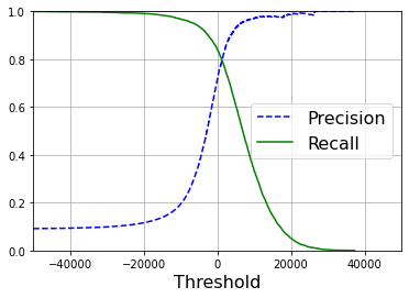
Accuracy/recall tradeoff
Scikit-learn s cannot directly set the threshold for F1score, but can access the decision scores it uses to predict. As shown below
y_scores = sgd_clf.decision_function([some_digit])
y_scores
array([1066.49326077])
threshold = 0
y_some_digit_pred = (y_scores > threshold)
y_some_digit_pred
array([ True])
threshold = 1100
y_some_digit_pred = (y_scores > threshold)
y_some_digit_pred
array([False])
The threshold used by the SGDClassifier classifier demonstrates that increasing the threshold reduces the recall rate.
Here's how to score all the instances in the training set
y_scores = cross_val_predict(sgd_clf,X_train,y_train_5,cv=3,method="decision_function")
#Accuracy and recall rate for calculating all possible thresholds
from sklearn.metrics import precision_recall_curve
precisions,recalls,thresholds = precision_recall_curve(y_train_5,y_scores)

#Use Matplotlib to plot function diagrams of accuracy and recall relative to thresholds
def plot_precision_recall_vs_threshold(precision,recalls,thresholds):
    plt.plot(thresholds,precision[:-1],"b--",label="Precision")
    plt.plot(thresholds,recalls[:-1],"g-",label="Recall")
    plt.legend(loc="center right", fontsize=16)
    plt.xlabel("Threshold", fontsize=16)
    plt.grid(True)
    plt.axis([-50000, 50000, 0, 1])

plot_precision_recall_vs_threshold(precisions,recalls,thresholds)
plt.show()
#Function Diagram of Accuracy Recall Rate
def plot_precision_vs_recall(precisions, recalls):
    plt.plot(recalls, precisions, "b-", linewidth=2)
    plt.xlabel("Recall", fontsize=16)
    plt.ylabel("Precision", fontsize=16)
    plt.axis([0, 1, 0, 1])
    plt.grid(True)
recall_90_precision = recalls[np.argmax(precisions >= 0.90)]
plt.figure(figsize=(8, 6))
plot_precision_vs_recall(precisions, recalls)
plt.plot([recall_90_precision, recall_90_precision], [0., 0.9], "r:")
plt.plot([0.0, recall_90_precision], [0.9, 0.9], "r:")
plt.plot([recall_90_precision], [0.9], "ro")
plt.show()
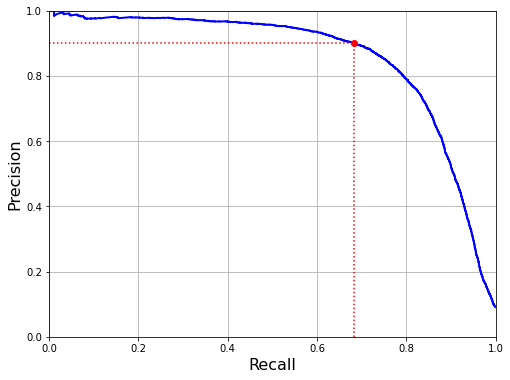
#Set precision to 90%

threshold_90_precision = thresholds[np.argmax(precisions >= 0.90)]
y_train_pred_90 = (y_scores >= threshold_90_precision)
precision_score(y_train_5,y_train_pred_90)
0.9001457725947521
recall_score(y_train_5,y_train_pred_90)
0.6834532374100719
So if someone needs 99% accuracy for you, you can ask, "What is the recall rate?" Killing him is a surprise.
ROC Curve
The ROC curve plots the true class rate (also recall rate) versus the false positive class rate (FPR), which is the ratio of negative class instances misclassified as positive = 1-TNR
ROC curves plot the relationship between sensitivity (recall) and (1-specificity)
from sklearn.metrics import roc_curve
fpr,tpr,threshold = roc_curve(y_train_5,y_scores)

def plot_roc_curve(fpr,tpr,label = None):
    plt.plot(fpr,tpr,linewidth=2,label=label)
    plt.plot([0,1],[0,1],'k--')
    plt.axis([0, 1, 0, 1])
    plt.xlabel('False Positive Rate (Fall-Out)', fontsize=16)
    plt.ylabel('True Positive Rate (Recall)', fontsize=16)
    plt.grid(True)

plot_roc_curve(fpr,tpr)
plt.show()
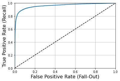
Another way to compare classifiers is to measure the area under the curve (AUC), perfect AUC=1, and pure random classifier AUC=0.5
from sklearn.metrics import roc_auc_score
roc_auc_score(y_train_5,y_scores)
Selection of ROC Curve and PR Curve0.9604387033143528
When positive classes are very rare or you are more concerned with positive classes than with false negative classes, choose PR curves, or ROC curves instead.
Random Forest Classifier
from sklearn.ensemble import RandomForestClassifier

forest_clf = RandomForestClassifier(random_state=27)
y_probas_forest =cross_val_predict(forest_clf,X_train,y_train_5,cv=3,method="predict_proba")
y_scores_forest = y_probas_forest[:,1]
fpr_forest,tpr_forest,thresholds_forest = roc_curve(y_train_5,y_scores_forest)

plt.plot(fpr,tpr,"b:",label="SGD")
plot_roc_curve(fpr_forest,tpr_forest,"Random forest")
plt.legend(loc="lower right")
plt.show()
[External chain picture transfer failed, source station may have anti-theft chain mechanism, it is recommended to save the picture and upload it directly (img-jkTeibfC-1638890528716)(output_46_0.png)]
roc_auc_score(y_train_5,y_scores_forest)
0.9983414796223264
RandomForestClassifier's ROC curve looks much better than SGDClassifier's, it's closer to the upper left corner, so its ROC-AUC score is much higher
multi-class classifier
The Multiclassifier is divided into OvO and OvR, where OvO is used, that is, the Multiclassifier here actually classifies 45 binary classifiers
from sklearn.svm import SVC

svm_clf = SVC()
svm_clf.fit(X_train,y_train)
svm_clf.predict([some_digit])
array([5], dtype=uint8)
some_digit_scores = svm_clf.decision_function([some_digit])
some_digit_scores
array([[ 1.72501977,  2.72809088,  7.2510018 ,  8.3076379 , -0.31087254,
         9.3132482 ,  1.70975103,  2.76765202,  6.23049537,  4.84771048]])
The top score is really 5
np.argmax(some_digit_scores)
5
When training a classifier, a list of target classes is stored in the classes attribute, sorted by the size of the values
svm_clf.classes_
array([0, 1, 2, 3, 4, 5, 6, 7, 8, 9], dtype=uint8)
If you want to force Scikit-learn s to use one-to-one or one-to-one residual policies, you can use either the OneVsOneClasssifier or the OneVsRestClassifier class.
from sklearn.multiclass import OneVsRestClassifier

ovr_clf = OneVsRestClassifier(SVC())
ovr_clf.fit(X_train,y_train)
ovr_clf.predict([some_digit])
array([5], dtype=uint8)
len(ovr_clf.estimators_)
10
The multiclass problem of training SGDClassifier or RandomForestClassifier is similar to the one above
sgd_clf.fit(X_train,y_train)
sgd_clf.predict([some_digit])
#SGD classifiers can directly divide instances into multiple classes, so you don't have to decide whether to OvO or OvR
array([3], dtype=uint8)
sgd_clf.decision_function([some_digit])
array([[-16594.39761568, -22903.10175344, -15146.89058029,
          1185.04960985, -20053.1928768 ,    508.90204236,
        -23168.38978204, -19229.31273118, -10995.42427777,
         -5902.26098972]])
To evaluate this classifier, as always, use cross-validation to evaluate
cross_val_score(sgd_clf,X_train,y_train,cv=3,scoring="accuracy")
array([0.8714 , 0.8818 , 0.86235])
Simple scaling of the input further improves accuracy
from sklearn.preprocessing import StandardScaler
scaler = StandardScaler()
X_train_scaled = scaler.fit_transform(X_train.astype(np.float64))
cross_val_score(sgd_clf,X_train_scaled,y_train,cv=3,scoring="accuracy")
array([0.90025, 0.89075, 0.901 ])
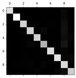
error analysis
If you want to further improve the model, one way to do this is to analyze its error type, first look at the confusion matrix
y_train_pred = cross_val_predict(sgd_clf,X_train_scaled,y_train,cv=3)
conf_mx = confusion_matrix(y_train,y_train_pred)
conf_mx
array([[5572,    0,   23,    6,    9,   48,   36,    6,  222,    1],
       [   0, 6399,   39,   21,    4,   44,    4,    7,  214,   10],
       [  27,   27, 5243,   90,   71,   24,   65,   36,  368,    7],
       [  22,   17,  117, 5217,    2,  209,   26,   39,  411,   71],
       [  10,   14,   48,    8, 5190,   12,   35,   24,  338,  163],
       [  26,   15,   29,  167,   54, 4449,   73,   14,  536,   58],
       [  30,   15,   46,    2,   44,   96, 5547,    3,  134,    1],
       [  20,   11,   50,   25,   49,   12,    3, 5692,  192,  211],
       [  16,   65,   51,   89,    3,  126,   24,   10, 5425,   42],
       [  21,   18,   30,   61,  116,   36,    1,  178,  382, 5106]],
      dtype=int64)
Many numbers seem cumbersome and are presented using matshow() from matplotlib
plt.matshow(conf_mx,cmap=plt.cm.gray)
plt.show()
Compare Error Rate
row_sums = conf_mx.sum(axis=1,keepdims = True)
norm_conf_mx = conf_mx / row_sums
Fill the diagonal with 0, keep errors, redraw the results
np.fill_diagonal(norm_conf_mx,0)
plt.matshow(norm_conf_mx,cmap=plt.cm.gray)
plt.show()

Analyzing confusion matrices often helps you gain insight into how to improve your classifier.