Jupyter notebook of this case: click here .
For the travel of sharing bicycles, each travel can be regarded as a travel process from the beginning to the end. When we regard the starting point and the ending point as nodes and the travel between them as edges, we can build a network. By analyzing this network, we can get information about the spatial structure of the city and the macro travel characteristics of shared bicycle demand.
Community discovery, also known as graph segmentation, helps us reveal the hidden relationship between nodes in the network. In this example, we will introduce how to integrate TransBigData into the community discovery analysis process of sharing bicycle data.
import pandas as pd
import numpy as np
import geopandas as gpd
import transbigdata as tbd
Data preprocessing
Before community discovery, we first need to preprocess the data. Extract the travel OD from the shared single vehicle order, eliminate the abnormal travel, and take the cleaned data as the research object.
#Read shared vehicle data
bikedata = pd.read_csv(r'data/bikedata-sample.csv')
bikedata.head(5)
| BIKE_ID | DATA_TIME | LOCK_STATUS | LONGITUDE | LATITUDE | |
|---|---|---|---|---|---|
| 0 | 5 | 2018-09-01 0:00:36 | 1 | 121.363566 | 31.259615 |
| 1 | 6 | 2018-09-01 0:00:50 | 0 | 121.406226 | 31.214436 |
| 2 | 6 | 2018-09-01 0:03:01 | 1 | 121.409402 | 31.215259 |
| 3 | 6 | 2018-09-01 0:24:53 | 0 | 121.409228 | 31.214427 |
| 4 | 6 | 2018-09-01 0:26:38 | 1 | 121.409771 | 31.214406 |
Read the boundary of the study area and use TBD clean_ The outofshape method eliminates data outside the study area
#Read the boundary of Shanghai Administrative Division
shanghai_admin = gpd.read_file(r'data/shanghai.json')
#Exclude data outside the scope of the study
bikedata = tbd.clean_outofshape(bikedata, shanghai_admin, col=['LONGITUDE', 'LATITUDE'], accuracy=500)
Use TBD bikedata_ to_ OD method identifies travel OD information from single vehicle data
#Identify single vehicle travel OD
move_data,stop_data = tbd.bikedata_to_od(bikedata,
                   col = ['BIKE_ID','DATA_TIME','LONGITUDE','LATITUDE','LOCK_STATUS'])
move_data.head(5)| BIKE_ID | stime | slon | slat | etime | elon | elat | |
|---|---|---|---|---|---|---|---|
| 96 | 6 | 2018-09-01 0:00:50 | 121.406226 | 31.214436 | 2018-09-01 0:03:01 | 121.409402 | 31.215259 |
| 561 | 6 | 2018-09-01 0:24:53 | 121.409228 | 31.214427 | 2018-09-01 0:26:38 | 121.409771 | 31.214406 |
| 564 | 6 | 2018-09-01 0:50:16 | 121.409727 | 31.214403 | 2018-09-01 0:52:14 | 121.412610 | 31.214905 |
| 784 | 6 | 2018-09-01 0:53:38 | 121.413333 | 31.214951 | 2018-09-01 0:55:38 | 121.412656 | 31.217051 |
| 1028 | 6 | 2018-09-01 11:35:01 | 121.419261 | 31.213414 | 2018-09-01 11:35:13 | 121.419518 | 31.213657 |
We need to eliminate long and short bike sharing trips. Use TBD Getdistance obtains the straight-line distance between the start and end points, and filters and deletes trips with a straight-line distance of less than 100m and more than 10km
#Calculate the riding straight distance
move_data['distance'] = tbd.getdistance(move_data['slon'],move_data['slat'],move_data['elon'],move_data['elat'])
#Clean the riding data and delete long and short trips
move_data = move_data[(move_data['distance']>100)&(move_data['distance']<10000)]
Next, we take 500 meters × The 500m grid is the smallest analysis unit, using TBD grid_ The params method obtains the grid division parameters, and then inputs the parameters into TBD odagg_ Grid method for grid aggregation of OD
# Get grid partition parameters
bounds = (120.85, 30.67, 122.24, 31.87)
params = tbd.grid_params(bounds,accuracy = 500)
#Aggregate OD
od_gdf = tbd.odagg_grid(move_data, params, col=['slon', 'slat', 'elon', 'elat'])
od_gdf.head(5)
| SLONCOL | SLATCOL | ELONCOL | ELATCOL | count | SHBLON | SHBLAT | EHBLON | EHBLAT | geometry | |
|---|---|---|---|---|---|---|---|---|---|---|
| 0 | 26 | 95 | 26 | 96 | 1 | 120.986782 | 31.097177 | 120.986782 | 31.101674 | LINESTRING (120.98678 31.09718, 120.98678 31.1... |
| 40803 | 117 | 129 | 116 | 127 | 1 | 121.465519 | 31.250062 | 121.460258 | 31.241069 | LINESTRING (121.46552 31.25006, 121.46026 31.2... |
| 40807 | 117 | 129 | 117 | 128 | 1 | 121.465519 | 31.250062 | 121.465519 | 31.245565 | LINESTRING (121.46552 31.25006, 121.46552 31.2... |
| 40810 | 117 | 129 | 117 | 131 | 1 | 121.465519 | 31.250062 | 121.465519 | 31.259055 | LINESTRING (121.46552 31.25006, 121.46552 31.2... |
| 40811 | 117 | 129 | 118 | 126 | 1 | 121.465519 | 31.250062 | 121.470780 | 31.236572 | LINESTRING (121.46552 31.25006, 121.47078 31.2... |
The results of OD aggregation are visualized on the map with TBD plot_ Map load the map basemap and use TBD Plot scale add scale bar and north arrow
#Plot Frame
import matplotlib.pyplot as plt
import plot_map
fig =plt.figure(1,(8,8),dpi=300)
ax =plt.subplot(111)
plt.sca(ax)
#Add map basemap
tbd.plot_map(plt,bounds,zoom = 11,style = 8)
#Draw colorbar
cax = plt.axes([0.05, 0.33, 0.02, 0.3])
plt.title('Data count')
plt.sca(ax)
#Draw OD
od_gdf.plot(ax = ax,column = 'count',cmap = 'Blues_r',linewidth = 0.5,vmax = 10,cax = cax,legend = True)
#Add scale bar and north arrow
tbd.plotscale(ax,bounds = bounds,textsize = 10,compasssize = 1,textcolor = 'white',accuracy = 2000,rect = [0.06,0.03],zorder = 10)
plt.axis('off')
plt.xlim(bounds[0],bounds[2])
plt.ylim(bounds[1],bounds[3])
plt.show()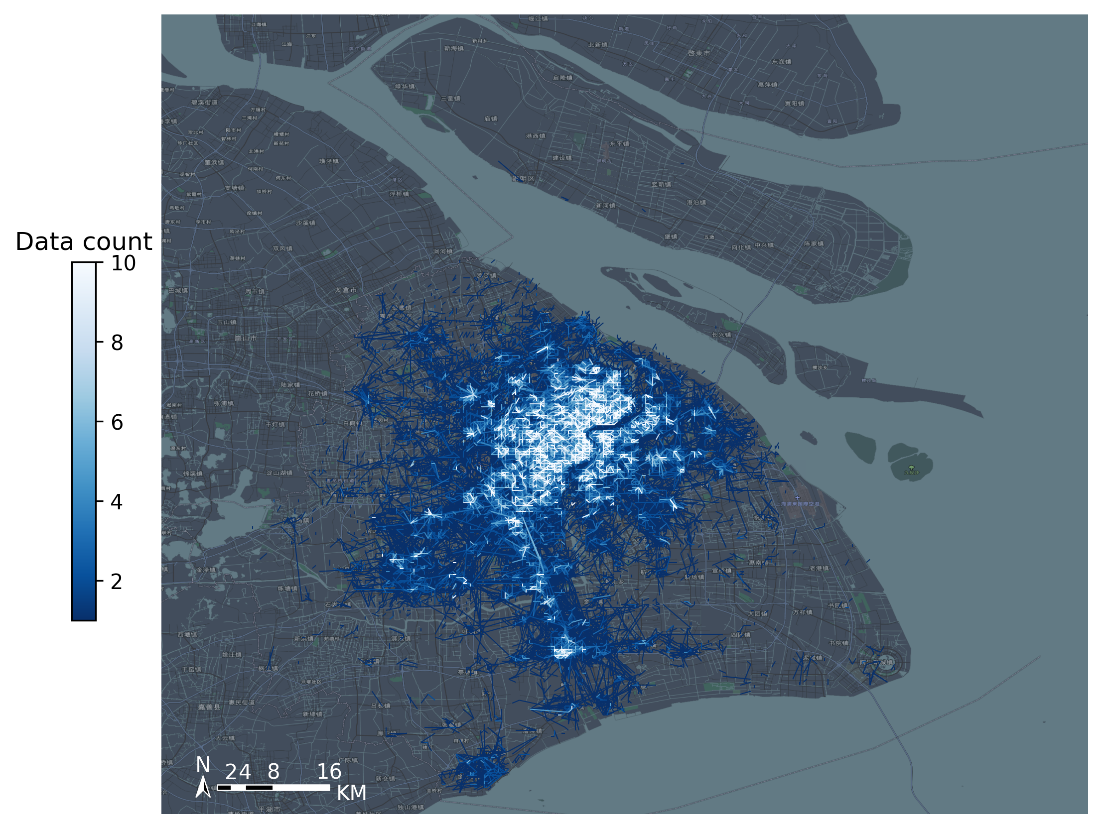
Extract node information
Use the igraph package to build the network. In Python, the function of igraph is similar to that of networkx. They both provide the function of network analysis, but only differ in the support of some algorithms. When building a network, we need to provide information about the nodes and edges of the network to igraph. Take each grid appearing in OD data as a node. When building node information, you need to create a numeric number starting from 0 for the node. The code is as follows
#Change the longitude and latitude grid number of the start and end points into a field
od_gdf['S'] = od_gdf['SLONCOL'].astype(str) + ',' + od_gdf['SLATCOL'].astype(str)
od_gdf['E'] = od_gdf['ELONCOL'].astype(str) + ',' + od_gdf['ELATCOL'].astype(str)
#Extract node set
node = set(od_gdf['S'])|set(od_gdf['E'])
#Turn node collection into DataFrame
node = pd.DataFrame(node)
#Renumber nodes
node['id'] = range(len(node))
node
| 0 | id | |
|---|---|---|
| 0 | 118,134 | 0 |
| 1 | 109,102 | 1 |
| 2 | 59,71 | 2 |
| 3 | 93,78 | 3 |
| 4 | 96,17 | 4 |
| ... | ... | ... |
| 9806 | 94,97 | 9806 |
| 9807 | 106,152 | 9807 |
| 9808 | 124,134 | 9808 |
| 9809 | 98,158 | 9809 |
| 9810 | 152,86 | 9810 |
9811 rows × 2 columns
Extract edge information
Connect the new number to the OD information table to extract the travel volume between the new ID S
#Connect the new number to the OD data
node.columns = ['S','S_id']
od_gdf = pd.merge(od_gdf,node,on = ['S'])
node.columns = ['E','E_id']
od_gdf = pd.merge(od_gdf,node,on = ['E'])
#Extract edge information
edge = od_gdf[['S_id','E_id','count']]
edge
| S_id | E_id | count | |
|---|---|---|---|
| 0 | 8261 | 7105 | 1 |
| 1 | 9513 | 2509 | 1 |
| 2 | 118 | 2509 | 3 |
| 3 | 348 | 2509 | 1 |
| 4 | 1684 | 2509 | 1 |
| ... | ... | ... | ... |
| 68468 | 8024 | 4490 | 2 |
| 68469 | 4216 | 3802 | 2 |
| 68470 | 4786 | 6654 | 2 |
| 68471 | 6484 | 602 | 3 |
| 68472 | 7867 | 8270 | 3 |
68473 rows × 3 columns
Build network
Import the igraph package, create the network, add nodes, and input the edge data into the network. At the same time, add corresponding weights for each edge
import igraph
#Create network
g = igraph.Graph()
#Add nodes to the network.
g.add_vertices(len(node))
#Add edges to the network.
g.add_edges(edge[['S_id','E_id']].values)
#Extract the weights of the edges.
edge_weights = edge[['count']].values
#Add weights to edges.
for i in range(len(edge_weights)):
    g.es[i]['weight'] = edge_weights[i]
Community discovery
The community discovery algorithm is applied to the constructed network. Among them, we use the g.community that comes with the igraph package_ The multi-level method implements the Fast unfolding community discovery algorithm. As we introduced earlier, the Fast unfolding algorithm combines communities iteratively layer by layer until the modularity is optimal_ Return can be set in the multilevel method_ Levels returns the intermediate result of the iteration. Here we set return_levels is False, and only the final result is returned for analysis
#Community discovery
g_clustered = g.community_multilevel(weights = edge_weights, return_levels=False)
The results of community discovery are stored in G_ In the clustered variable, you can use the built-in method to directly calculate the modularity
#Modularity
g_clustered.modularity
0.8496561130926571
Generally speaking, the modularity above 0.5 already belongs to a high value. The modularity of this result reaches 0.84, indicating that the community structure of the network is very obvious, and the community division result can also divide the network well. Next, we assign the community division results to the node information table to prepare for the following visualization. The code is as follows
#Assign the result to the node
node['group'] = g_clustered.membership
#Heavy life list
node.columns = ['grid','node_id','group']
node
| grid | node_id | group | |
|---|---|---|---|
| 0 | 118,134 | 0 | 0 |
| 1 | 109,102 | 1 | 1 |
| 2 | 59,71 | 2 | 2 |
| 3 | 93,78 | 3 | 3 |
| 4 | 96,17 | 4 | 4 |
| ... | ... | ... | ... |
| 9806 | 94,97 | 9806 | 8 |
| 9807 | 106,152 | 9807 | 36 |
| 9808 | 124,134 | 9808 | 37 |
| 9809 | 98,158 | 9809 | 9 |
| 9810 | 152,86 | 9810 | 26 |
9811 rows × 3 columns
Community visualization
In the results of community discovery, there may be only a small number of nodes in some communities, which can not form a large-scale community. These communities are outliers and should be deleted before visualization. Here we keep communities with more than 10 grids
#Count the number of grids per community
group = node['group'].value_counts()
#Extract communities larger than 10 grids
group = group[group>10]
#Keep only the grids of these communities
node = node[node['group'].apply(lambda r:r in group.index)]
Restore the grid number and use TBD gridid_ to_ The polygon method generates the geographic geometry of the grid from the grid number
#Get grid number by segmentation
node['LONCOL'] = node['grid'].apply(lambda r:r.split(',')[0]).astype(int)
node['LATCOL'] = node['grid'].apply(lambda r:r.split(',')[1]).astype(int)
#Generate Grid Geographic graphics
node['geometry'] = tbd.gridid_to_polygon(node['LONCOL'],node['LATCOL'],params)
#Convert to GeoDataFrame
import geopandas as gpd
node = gpd.GeoDataFrame(node)
node| grid | node_id | group | LONCOL | LATCOL | geometry | |
|---|---|---|---|---|---|---|
| 0 | 118,134 | 0 | 0 | 118 | 134 | POLYGON ((121.46815 31.27030, 121.47341 31.270... |
| 1 | 109,102 | 1 | 1 | 109 | 102 | POLYGON ((121.42080 31.12641, 121.42606 31.126... |
| 3 | 93,78 | 3 | 3 | 93 | 78 | POLYGON ((121.33663 31.01849, 121.34189 31.018... |
| 4 | 96,17 | 4 | 4 | 96 | 17 | POLYGON ((121.35241 30.74419, 121.35767 30.744... |
| 5 | 156,117 | 5 | 5 | 156 | 117 | POLYGON ((121.66806 31.19385, 121.67332 31.193... |
| ... | ... | ... | ... | ... | ... | ... |
| 9806 | 94,97 | 9806 | 8 | 94 | 97 | POLYGON ((121.34189 31.10392, 121.34715 31.103... |
| 9807 | 106,152 | 9807 | 36 | 106 | 152 | POLYGON ((121.40502 31.35124, 121.41028 31.351... |
| 9808 | 124,134 | 9808 | 37 | 124 | 134 | POLYGON ((121.49971 31.27030, 121.50498 31.270... |
| 9809 | 98,158 | 9809 | 9 | 98 | 158 | POLYGON ((121.36293 31.37822, 121.36819 31.378... |
| 9810 | 152,86 | 9810 | 26 | 152 | 86 | POLYGON ((121.64702 31.05446, 121.65228 31.054... |
8527 rows × 6 columns
In this step, we restore each node to a grid, mark the community number to which the node belongs, generate the geographic information of each grid, and convert it into a GeoDataFrame. We can draw the grid with the following code to test whether the generation is successful
node.plot('group')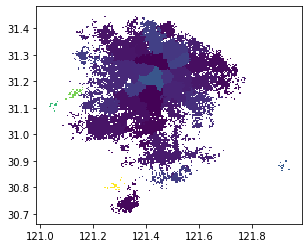
Here, we map the group number of the group field to the color for preliminary visualization. The colors of different groups are different. It can be seen from the graph of the result that most grids of the same color are clustered together in geospatial space, indicating that the spatial connection of sharing bicycles can closely connect the close areas in geospatial space
The visualization effect of the previous results is not obvious. We can't clearly see the partition from the figure. Next, we can adjust and visualize the partition results. The adjustment of visualization mainly includes the following ideas:
-
A more appropriate zoning result should be that each region is spatially continuous. In the preliminary visualization results, many grids exist in isolation in space, and these points should be eliminated.
-
In the visualization results, we can merge the grids of the same group to form face features for each partition, so that the boundary of the partition can be drawn in the next visualization.
-
In the zoning results, there may be "enclaves" of other regions in some regions, that is, they belong to this partition but are surrounded by other partitions. They can only "fly" through the possessions of other partitions to reach their own enclaves. This kind of zoning is also difficult to manage in the actual operation of sharing bicycles, which should be avoided.
To solve the above problems, we can use two GIS processing methods provided by TransBigData, TBD merge_ Polygon and TBD polyon_ exterior. TBD merge_ Polygon can merge face features of the same group, while TBD polyon_ Exterior can take the outer boundary of the polygon and then form a new polygon to eliminate the enclave. At the same time, you can also set the minimum area to eliminate face features smaller than this area. The code is as follows
#Combine the face features of the same group by grouping the group field
node_community = tbd.merge_polygon(node,'group')
#Input polygon GeoDataFrame data and take the outer boundary of the polygon to form a new polygon
#Set the minimum area minarea to eliminate all faces smaller than this area to avoid a large number of outliers
node_community = tbd.polyon_exterior(node_community,minarea = 0.000100)
After processing the face features of the community, you need to visualize the face features. We want to give different colors to different faces. In the visualization chapter, we mentioned that when there is no numerical difference between the displayed elements, the color selection needs to keep their respective colors with the same brightness and saturation. seaborn's palette method can quickly generate multiple colors under the same brightness and saturation
#Generate palette
import seaborn as sns
## l: Brightness
## s: Saturation
cmap = sns.hls_palette(n_colors=len(node_community), l=.7, s=0.8)
sns.palplot(cmap)

Visualize community results
#Plot Frame
import matplotlib.pyplot as plt
import plot_map
fig =plt.figure(1,(8,8),dpi=300)
ax =plt.subplot(111)
plt.sca(ax)
#Add map basemap
tbd.plot_map(plt,bounds,zoom = 10,style = 6)
#Set colormap
from matplotlib.colors import ListedColormap
#Disrupt the order of the community
node_community = node_community.sample(frac=1)
#Draw community
node_community.plot(cmap = ListedColormap(cmap),ax = ax,edgecolor = '#333',alpha = 0.8)
#Add scale bar and north arrow
tbd.plotscale(ax,bounds = bounds,textsize = 10,compasssize = 1,textcolor = 'k'
              ,accuracy = 2000,rect = [0.06,0.03],zorder = 10)
plt.axis('off')
plt.xlim(bounds[0],bounds[2])
plt.ylim(bounds[1],bounds[3])
plt.show()
So far, we have successfully visualized the shared bicycle community and mapped the boundary of each community. When the community discovery model is used for zoning, no geospatial information is input into the model, and the segmentation of the study area only depends on the network connection composed of shared single vehicle travel demand.