1 understanding of simulated annealing
As a heuristic search method, simulated annealing is different from Monte Carlo method, enumeration method and other blind search methods, that is, it can use the information in the search process to improve the search strategy. Therefore, the characteristic of heuristic search method is that it helps to speed up the solution process. It can find a better solution, but it may not find the optimal solution, This conclusion will be explained later.
1.1 mountain climbing method
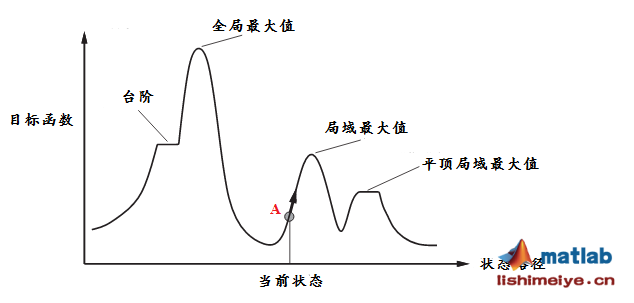
As a local optimization algorithm, the main steps of mountain climbing method are as follows:
(1) An initial solution is randomly generated in the solution space;
(2) At the position of the initial solution, advance one step to the left neighborhood and the right domain respectively;
(3) Compare the objective function values under different walking methods, and select the traveling direction according to the required minimum value requirements;
(4) Repeat the above operations until a local maximum point is found and the search ends.
From the above figure, it can be seen that if the selected position of point A of the initial solution directly affects the final optimization result, taking the state in the figure as an example, point A will eventually find the local maximum and miss the global maximum. Therefore, this is the defect of mountain climbing. It is analyzed that the mountain climbing method falls into the trap of local optimization, mainly because it directly discards the temporarily unsatisfactory solution when looking for A new solution. According to this step, the scope of the solution is getting smaller and smaller, which is A bit greedy algorithm. Therefore, the key to solve the mountain climbing method is to accept the new unsatisfactory solution with A certain probability.
1.2 idea of solving function maximum value problem
Use the above ideas to solve the function maximum value problem:
(1) Randomly find a new solution xj near the initial solution xi, and the corresponding function value is f(xj). Compare the function values f(xi) and f(xj) by case;
(2) If f (XJ) > F (XI), accept the new solution, replace the original initial solution with the new solution, and continue the cycle;
(3) If f(xj) < f(xi), the new solution is accepted with an acceptable probability p, and the new solution replaces the original solution to continue the cycle. Probability p ∈ [0,1], the closer the values of f(xi) and f(xj), the greater P.
Therefore, the key to the problem is to find a function that meets the requirements to describe p. From the above, p is proportional to.
If you look for a function with a value range of [0,1], and the function value y is inversely proportional to | f(xj)-f(xi) |, it is easy to think of an exponential function
y
=
e
−
∣
f
(
x
j
)
−
f
(
x
i
)
∣
y=e^{-|f(xj)-f(xi)|}
y=e−∣f(xj)−f(xi)∣
In order to continue the constructor, we need to further understand the probability p:
(1) The greater the probability of accepting the new solution, the larger the search range of the solution in space;
(2) In the whole solution search process, the search range of the early solution should be as large as possible to avoid falling into the local optimal solution, while the search range in the later stage needs to be smaller.
Therefore, the constructed probability function p should be
y
=
e
−
∣
f
(
x
j
)
−
f
(
x
i
)
∣
×
C
t
y=e^{-|f(xj)-f(xi)|×C_t}
y=e−∣f(xj)−f(xi)∣×Ct
Where Ct is a function of time t. The longer the time, the greater the Ct.
The above functions are substituted into the idea of solving the maximum value of the function, and the solution process is as follows:
(1) Randomly generate an initial solution A and calculate the function value f(A) corresponding to solution A;
(2) A solution B is randomly generated near position a, and the function value f(B) of solution B is calculated. The size fraction of the comparison between f(A) and f(B) is discussed;
(3) If f(B) > f(A), assign solution B to A, and then repeat the above steps; If f(B) ≤ f(A), calculate the probability of accepting B
y
=
e
−
∣
f
(
x
j
)
−
f
(
x
i
)
∣
×
C
t
y=e^{-|f(xj)-f(xi)|×C_t}
y=e−∣f(xj)−f(xi)∣ × Ct , then randomly generate A number r between [0,1]. If R < p, assign solution B to A, and then repeat the above steps; Otherwise, continue with step (2) and continue.
In the above operations, there are several key points that need special attention:
(1) How to set Ct function
Ct function is constructed by the unique temperature drop formula in simulated annealing, in which the temperature drop formula is:
T
t
+
1
=
α
T
t
T_{t+1} = \alpha T_t
Tt+1= α TT ﹐ where α The range of is [0,1], α Take 0.95, so the temperature at time t is:
T
t
=
α
t
T
0
T_t = \alpha ^t T_0
Tt= α T0 ^ take
C
t
=
1
T
t
=
1
α
t
T
0
C_t = \frac{1}{T_t} =\frac{1}{ \alpha ^t T_0}
Ct=Tt1=αtT01
It can be seen from the above that Ct is a monotonically increasing function about t, so the Ct function constructed above meets the requirements. The expression of probability p is:
p
t
=
e
−
∣
f
(
B
)
−
f
(
A
)
∣
T
t
p_t = e^-\frac{|f(B)-f(A)|}{T_t}
pt=e−Tt∣f(B)−f(A)∣
(2) Loop and end condition of the search process
In order to ensure the thoroughness of the search process, multiple searches are required at the same temperature; After reaching the set search times, reduce the temperature and start a new cycle again.
As for the end conditions of the search process, there are generally three types:
(a) The number of specified iterations has been reached; (b) The specified falling temperature is reached; (c) The value of the optimal solution does not change after M iterations.
(3) How to generate new solutions is the most important part
The method of how to generate new solutions can only be analyzed in detail.
Taking solving the function maximum problem as an example, the new solution is generated by the function in Matlab. The specific rules for generating new solutions are as follows:
Suppose the current solution is
X
=
(
x
1
,
x
2
,
.
.
.
,
x
n
)
X=(x_1,x_2,...,x_n)
X=(x1, x2,..., xn) first generate a set of random numbers
Y
=
(
y
1
,
y
2
,
.
.
.
,
y
n
)
Y=(y_1,y_2,...,y_n)
Y=(y1, y2,..., yn) where y obeys N(0,1), and Y is standardized to obtain
Z
=
(
z
1
,
z
2
,
.
.
.
,
z
n
)
Z=(z_1,z_2,...,z_n)
Z=(z1, z2,..., zn) where
z
t
=
y
i
y
1
2
+
y
2
2
+
.
.
.
+
y
n
2
z_t = \frac {y_i}{\sqrt{y_1^2+y_2^2+...+y_n^2}}
zt=y12+y22+...+yn2
yi
Then proceed as follows:
(1) Calculation formula generated by the new solution:
x
i
n
e
w
=
x
i
+
T
×
z
i
x_i^{new}= x_i + T×z_i
xinew=xi+T×zi
(2) Check whether the new solution is within the upper and lower boundaries,
(a) if conditions are met
l
b
i
≤
x
i
n
e
w
≤
u
b
i
lb_i ≤ x_i^{new} ≤ ub_i
lbi ≤ xinew ≤ ubi , direct assignment with new solution
x
j
=
x
i
n
e
w
x_j = x_i^{new}
xj=xinew
(b) if conditions are met
x
i
n
e
w
<
l
b
i
x_i^{new} < lb_i
xinew < LBI , then the new solution is
x
j
=
r
×
l
b
i
+
(
1
−
r
)
×
x
i
x_j=r×lb_i + (1-r)×x_i
xj=r × lbi+(1−r) × xi, where R is a random number uniformly distributed in the interval [0,1];
(c) if conditions are met
x
i
n
e
w
>
u
b
i
x_i^{new} > ub_i
xinew > UBI , then the new solution is
x
j
=
r
×
u
b
i
+
(
1
−
r
)
×
x
i
x_j=r×ub_i+(1-r)×x_i
xj=r × ubi+(1−r) × xi, where R is a random number uniformly distributed in the interval [0,1].
2 example of solving the maximum value problem of function
2.1 title of single independent variable:
Find the maximum value of the function y=sin(x)+cos(5x) in the interval [- 1,1].
(1) Draw function
x=-1:0.01:1;
y=sin(x)+cos(5*x);
figure(1)
plot(x,y,'b');
hold on
(2) Parameter initialization
narvs =1; % Number of variables
T0 = 100; % initial temperature
T = T0; % The temperature will change during the iteration. The temperature is zero at the first iteration T0
maxgen = 500; % Maximum number of iterations
Lk = 200; % Number of iterations per temperature
alfa = 0.95; % Temperature attenuation coefficient
x_lb = -1; % x Lower bound of
x_ub = 1; % x Upper bound of
(3) Generate new solution
x0 = x_lb+(x_ub-x_lb)*rand(1,narvs);
h = scatter(x0,Obj_fun1(x0),'*r'); % scatter Is a function of drawing a two-dimensional scatter diagram, h Is a handle to the drawing
Where Obj_fun1 is the name of the function
(4) Save intermediate value
iter_x = x0;
iter_y = Obj_fun1(x0);
(5) Key points: simulated annealing process
for iter = 1:maxgen  %Outer loop, maximum number of iterations
    for i=1:Lk  % Internal circulation, number of iterations at each temperature
        %title(['Current temperature:',num2str(T)])
        y0 = Obj_fun1(x0);  % Calculates the function value of the current solution

        y = randn(1,narvs);  % Generate 1 line narvs Columnar N(0,1)Random number of
        z = y/sqrt(sum(y.^2));  % yes y Standardized treatment
        x_new = x0 + z*T;     %use Matlab Self contained function
        % If the position of the new solution exceeds the definition field, adjust it, that is, the operation corresponding to the above steps to generate a new solution
        for j =1:narvs
            if x_new(j) < x_lb(j)
                r = rand(1);
                x_new(j) = r*x_lb(j)+(1-r)*x0(j);
            elseif x_new(j) > x_ub(j)
                r =rand(1);
                x_new(j) = r*x_ub(j)+(1-r)*x0(j);
            end
        end
        x1 = x_new;
        y1 = Obj_fun1(x1);

        if y1 > y0 % The function value of the new solution is greater than the function value of the current solution

            x0 = x1; %Update current solution to new solution
            iter_x =[iter_x;x1];  % The newly found x1 Add to intermediate results
            iter_y =[iter_y;y1];  % The newly found y1 Add to intermediate results
        else
            p = exp(-(y0-y1)/T);  % according to Metropolis The criterion calculates a probability

            if rand(1) < p % Generate a random number and compare it with this probability. If the random number is less than this probability

                x0 = x1;
            end
        end

        h.XData = x0; % Update the handle of the scatter chart x Axis data
        h.YData = y0; % Update the handle of the scatter chart y Axis data
    end

    T = alfa * T;  % Temperature drop
    pause(0.01)  % Pause for a while before drawing
end
(6) Optimal solution output
[best_y,ind]=max(iter_y);  % Find the largest y Value and its subscript in the vector
best_x = iter_x(ind,:);  % Find the at this time according to the subscript x value
disp('The best location is:');disp(best_x)
disp('At this time, the optimal value is:');disp(best_y)

pause(1)
h.XData = [];h.YData = [];  % Delete the original scatter
scatter(best_x,best_y,'r');  % Re mark the scatter at the maximum
title(['The maximum value found by simulated annealing is',num2str(best_y)])  % Add the title above
(7) Simulation result diagram

The red circle represents the maximum value of the function in the [- 1,1] interval.
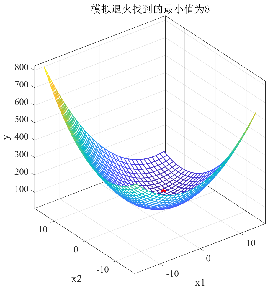
2.2 multiple independent variable questions:
Find function y = x 1 2 + x 2 2 − x 1 x 2 − 10 x 1 − 4 x 2 + 60 y=x_1^2+x_2^2-x_1x_2-10x_1-4x_2+60 Y = the minimum value of X12 + x22 − x1 − x2 − 10x1 − 4x2 + 60 within x1,x2 ∈ [- 15,15].
(1) Draw function
figure
x1 = -15:1:15;
x2 = -15:1:15;
[x1,x2] = meshgrid(x1,x2);
y = x1.^2 + x2.^2 - x1.*x2 - 10*x1 - 4*x2 + 60;
mesh(x1,x2,y)
xlabel('x1');  ylabel('x2');  zlabel('y');  % Label the axis
axis vis3d % Freeze the screen aspect ratio so that the rotation of a 3D object does not change the scale display of the coordinate axis
hold on  % Continue drawing on the drawing without closing the drawing
(2) Parameter initialization
narvs = 2; % Number of variables
T0 = 100;   % initial temperature
T = T0; % The temperature will change during the iteration. The temperature is zero at the first iteration T0
maxgen = 200;  % Maximum number of iterations
Lk = 100;  % Number of iterations per temperature
alfa = 0.95;  % Temperature attenuation coefficient
x_lb = [-15 -15]; % x Lower bound of
x_ub = [15 15]; % x Upper bound of
(3) Generate initial solution
x0 = zeros(1,narvs);
for i = 1: narvs
    x0(i) = x_lb(i) + (x_ub(i)-x_lb(i))*rand(1);
end
y0 = Obj_fun2(x0); % Calculates the function value of the current solution
h = scatter3(x0(1),x0(2),y0,'*r');  % scatter3 Is a function for drawing a three-dimensional scatter chart (returned here) h In order to get the handle of the graph, we will update its position in the future)
(4) Save intermediate quantity
min_y = y0;     % The function value corresponding to the best solution found by initialization is y0
MINY = zeros(maxgen,1); % Record the results found at the end of each outer cycle min_y ((convenient for drawing)
(5) Key points: simulated annealing process
for iter = 1 : maxgen  % External circulation, What I use here is to specify the maximum number of iterations
    for i = 1 : Lk  % Internal circulation, starting iteration at each temperature
        y = randn(1,narvs);  % Generate 1 line narvs Columnar N(0,1)random number
        z = y / sqrt(sum(y.^2)); % yes y Values are standardized
        x_new = x0 + z*T; % Calculated according to the generation rules of the new solution x_new Value of
        % If the position of the new solution exceeds the definition domain, adjust it
        for j = 1: narvs
            if x_new(j) < x_lb(j)
                r = rand(1);
                x_new(j) = r*x_lb(j)+(1-r)*x0(j);
            elseif x_new(j) > x_ub(j)
                r = rand(1);
                x_new(j) = r*x_ub(j)+(1-r)*x0(j);
            end
        end
        x1 = x_new;    % The adjusted x_new Assign to new solution x1
        y1 = Obj_fun2(x1);  % Calculate the function value of the new solution
        if y1 < y0    % If the function value of the new solution is less than the function value of the current solution
            x0 = x1; % Update current solution to new solution
            y0 = y1;
        else
            p = exp(-(y1 - y0)/T); % according to Metropolis The criterion calculates a probability
            if rand(1) < p   % Generate a random number and compare it with this probability. If the random number is less than this probability
                x0 = x1;  % Update current solution to new solution
                y0 = y1;
            end
        end
        % Determine whether to update the best solution found
        if y0 < min_y  % If the current solution is better, update it
            min_y = y0;  % Update minimum y
            best_x = x0;  % Update the best found x
        end
    end
    MINY(iter) = min_y; % Save the smallest value found after the end of this round of external circulation y
    T = alfa*T;   % Temperature drop
    pause(0.02)  % After a pause(Unit: Second)Then draw the picture
    h.XData = x0(1);  % Update the handle of the scatter chart x Axis data (at this time, the position of the solution changes on the diagram)
    h.YData = x0(2); % Update the handle of the scatter chart y Axis data (at this time, the position of the solution changes on the diagram)
    h.ZData = Obj_fun2(x0);  % Update the handle of the scatter chart z Axis data (at this time, the position of particles changes on the graph)
end
(6) Find the best location
disp('The best location is:'); disp(best_x)
disp('At this time, the optimal value is:'); disp(min_y)

pause(0.5)
h.XData = [];  h.YData = [];  h.ZData = [];  % Delete the original scatter
scatter3(best_x(1), best_x(2), min_y,'*r');  % Re mark the scatter at the minimum value
title(['The minimum value found by simulated annealing is', num2str(min_y)])  % Add the title above

%% Draw the minimum number found after each iteration y Graphics for
figure
plot(1:maxgen,MINY,'b-');
xlabel('Number of iterations');
ylabel('y Value of');
toc
(7) Simulation results
3 example of solving traveling salesman problem
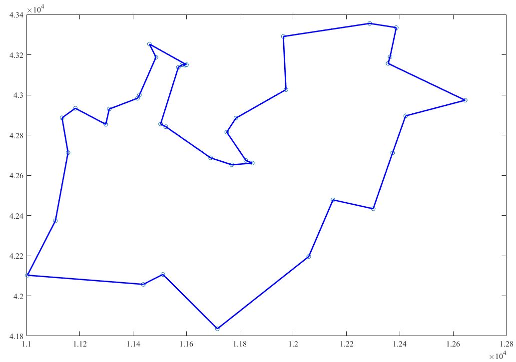
3.1 single traveler problem
Given the coordinate positions of 38 cities, the shortest loop to visit each city from the starting city and return to the starting city again is solved.
There are three methods to generate new path solutions:
(1) Exchange method: randomly select two nodes in the path and exchange the positions of the two points;
(2) Shift method: randomly select three nodes in the path and shift the point between the first two points to the third point;
(3) Inversion method: randomly select two nodes in the path and completely reverse the order between the points.
stsp.m code
(1) Load city coordinate location
coord = [11003.611100,42102.500000;11108.611100,42373.888900;11133.333300,42885.833300;11155.833300,42712.500000;11183.333300,42933.333300;11297.500000,42853.333300;11310.277800,42929.444400;11416.666700,42983.333300;11423.888900,43000.277800;11438.333300,42057.222200;11461.111100,43252.777800;11485.555600,43187.222200;11503.055600,42855.277800;11511.388900,42106.388900;11522.222200,42841.944400;11569.444400,43136.666700;11583.333300,43150.000000;11595.000000,43148.055600;11600.000000,43150.000000;11690.555600,42686.666700;11715.833300,41836.111100;11751.111100,42814.444400;11770.277800,42651.944400;11785.277800,42884.444400;11822.777800,42673.611100;11846.944400,42660.555600;11963.055600,43290.555600;11973.055600,43026.111100;12058.333300,42195.555600;12149.444400,42477.500000;12286.944400,43355.555600;12300.000000,42433.333300;12355.833300,43156.388900;12363.333300,43189.166700;12372.777800,42711.388900;12386.666700,43334.722200;12421.666700,42895.555600;12645.000000,42973.333300];
n = size(coord,1);  % Number of cities
figure  % Create a new graphics window
plot(coord(:,1),coord(:,2),'o');   % Draw a scatter map of the city
hold on % Wait a minute. I'm going to draw on this figure
(2) Calculate distance matrix
d = zeros(n);   % Initialize the distance matrix of two cities to 0
for i = 2:n
    for j = 1:i
        coord_i = coord(i,:);   x_i = coord_i(1);     y_i = coord_i(2);  % city i The abscissa of is x_i,The ordinate is y_i
        coord_j = coord(j,:);   x_j = coord_j(1);     y_j = coord_j(2);  % city j The abscissa of is x_j,The ordinate is y_j
        d(i,j) = sqrt((x_i-x_j)^2 + (y_i-y_j)^2);   % Computing City i and j Distance
    end
end
d = d+d';   % Generate the symmetrical side of the distance matrix
(3) Parameter initialization
T0 = 1000;   % initial temperature
T = T0; % The temperature will change during the iteration. The temperature is zero at the first iteration T0
maxgen = 1000;  % Maximum number of iterations
Lk = 500;  % Number of iterations per temperature
alpfa = 0.95;  % Temperature attenuation coefficient
(4) Generate initial solution
path0 = randperm(n);  % Generate a 1-n The randomly disrupted sequence is used as the initial path
result0 = calculate_tsp_d(path0,d); % Call what we wrote ourselves calculate_tsp_d Function to calculate the distance of the current path
(5) Save intermediate quantity
min_result = result0;     % The distance corresponding to the best solution found by initialization is result0
RESULT = zeros(maxgen,1); % Record the results found at the end of each outer cycle min_result ((convenient for drawing)
(6) Key points: simulated annealing process
for iter = 1 : maxgen  % External circulation, What I use here is to specify the maximum number of iterations
    for i = 1 : Lk  %  Internal circulation, starting iteration at each temperature
        path1 = gen_new_path(path0);  % Call what we wrote ourselves gen_new_path Function to generate a new path
        result1 = calculate_tsp_d(path1,d); % Calculate the distance of the new path
        %If the distance of the new solution is short, the value of the new solution is directly assigned to the original solution
        if result1 < result0
            path0 = path1; % Update current path to new path
            result0 = result1;
        else
            p = exp(-(result1 - result0)/T); % according to Metropolis The criterion calculates a probability
            if rand(1) < p   % Generate a random number and compare it with this probability. If the random number is less than this probability
                path0 = path1;  % Update current path to new path
                result0 = result1;
            end
        end
        % Determine whether to update the best solution found
        if result0 < min_result  % If the current solution is better, update it
            min_result = result0;  % Update minimum distance
            best_path = path0;  % Update the shortest path found
        end
    end
    RESULT(iter) = min_result; % Save the minimum distance found after the end of this round of external circulation
    T = alpfa*T;   % Temperature drop
end
(7) Output the optimal path and plot
disp('The best solution is:'); disp(mat2str(best_path))  % Convert numeric matrix to character vector
disp('At this time, the optimal value is:'); disp(min_result)


best_path = [best_path,best_path(1)];   % Add an element on the last side of the shortest path, that is, the first point (we want to generate a closed graph)
n = n+1;  % Number of cities plus one (following the previous step)
for i = 1:n-1
    j = i+1;
    coord_i = coord(best_path(i),:);   x_i = coord_i(1);     y_i = coord_i(2);
    coord_j = coord(best_path(j),:);   x_j = coord_j(1);     y_j = coord_j(2);
    plot([x_i,x_j],[y_i,y_j],'-b')    % Make a line segment at every two points until all the cities are finished
%     pause(0.02)  % Pause 0.02s Draw the next line segment
    hold on
end

%% Draw the graph of the shortest path found after each iteration
figure
plot(1:maxgen,RESULT,'b-');
xlabel('Number of iterations');
ylabel('Shortest path');

toc
3.2 multi traveling salesman problem
Multiple commodity salesmen have to go to several cities to sell goods. These salesmen are initially in the same city. They are assigned different paths. After passing through all cities, everyone returns to the starting city.
The first thing to think about is:
Suppose there are n+1 cities, 0 is the starting city, the numbers of other cities are 1 to N, and there are m travel agents in total, then the generated solution should be:
m-1 is a random sort composed of 0 and 1 to n.
Two points to note:
(1) When generating the initial solution, the randperm function is used to generate the random sorting of 1 to n, and then the randi function is used to randomly generate the position of inserting 0 again;
(2) When calculating the total distance or total cost, the solution needs to be split. The path passed by each traveler can be saved in a cell array.
However, there is still a problem when running according to the following code.
(1) Code for generating initial solution
path0 = randperm(n);  % The number of cities is n+1,Generate a 1-n The randomly disrupted sequence is used as the initial path
for i = 1:salesman_num-1
    len = length(path0);
    ind = randi(len);
    path0 = [path0(1:ind),0,path0(ind+1:end)];
end
(2) Clean up and split the generated solution_ path. m
function [cpath,k] = clear_path(path,salesman_num)
    cpath = cell(salesman_num,1);  % It is used to save the cities passed by each traveler participating in the work
    ind = find(path==0);  % Locate all split points
    k =1;  % Initialize counters, k Indicates the number of travel agents involved in the work
    for i=1:salesman_num-1
        if i==1 % If it is the first split point
            c = path(1:ind(i)-1); % Extract the city passed by the first traveler
        else
            c = path(ind(i-1)+1:ind(i)-1);  % Extract the city passed by the intermediate traveler
        end
        if ~isempty(c)
            cpath{k}=c;  % hold c Save to cell cpath The first k Location
            k =k+1;
        end
    end
    c = path(ind(end)+1:end);
    if ~isempty(c)
        cpath{k}=c;
    else
        k = k-1;
    end
    cpath = cpath(1:k);  % Only the anterior part of the cell is retained k A non empty part
end
(3) Calculate the cost corresponding to the current solution_ mtsp_ cost. m
function [cost,every_cost]=calculate_mtsp_cost(cpath,k,d)
    % To calculate the sum of the journey lengths of all travelers, you need to first calculate the journey length of each traveler
    every_cost =zeros(k,1);  % Initialize the journey length of each traveling salesman to 0
    for i=1:k
        path_i =cpath{i};  % The first i The route traveled by a traveler
        n = length(path_i); % The first i Number of cities traveled by a traveler
        for j =1:n
               if j == 1
                   every_cost(i)=every_cost(i)+d(1,path_i(j));
               else
                   every_cost(i)=every_cost(i)+d(path_i(j-1),path_i(j));
               end
        end
        every_cost(i)=every_cost(i)+d(path_i(end),1);
    end
    cost = sum(every_cost);
end
(4) The method of generating new solutions gen_new_path1.m
function path1 = gen_new_path1(path0,p1,p2)
    n = length(path0);
    r = rand(1);  % Randomly generate a[0,1]Uniformly distributed random number
    if r < p1  % Generate new path using exchange method
        c1 = randi(n);  % Generate 1-n A random integer in
        c2 = randi(n);  % Generate 1-n A random integer in
        path1 = path0;  % take path0 Value assigned to path1
        path1(c1)=path0(c2); % take path0 The first c2 The element of a position is assigned to path1 The first c1 Elements in multiple locations
        path1(c2)=path0(c1); % take path0 The first c1 The element of a position is assigned to path1 The first c2 Elements in multiple locations
    elseif r < p1+p2
        c1 = randi(n);  % Generate 1-n A random integer in
        c2 = randi(n);  % Generate 1-n A random integer in
        c3 = randi(n);  % Generate 1-n A random integer in
        sort_c = sort([c1 c2 c3]);  % yes c1,c2,c3 Sort from small to large
        c1 = sort_c(1);c2 = sort_c(2);c3 = sort_c(3);
        temp1 = path0(1:c1-1);
        temp2 = path0(c1:c2);
        temp3 = path0(c2+1:c3);
        temp4 = path0(c3+1:end);
        path1 = [temp1 temp3 temp2 temp4];
    else
        % A new path is generated by the inversion method
        c1 = randi(n);  % Generate 1-n A random integer in
        c2 = randi(n);  % Generate 1-n A random integer in c2;
        if c1 > c2
            tem = c2;
            c2 = c1;
            c1 = tem;
        end
        tem1 = path0(1:c1-1);
        tem2 = path0(c1:c2);
        tem3 = path0(c2+1:end);
        path1 = [tem1 fliplr(tem2) tem3];
    end
end
reference resources
The content of this paper refers to teacher Qingfeng's mathematical modeling simulated annealing video and the corresponding web page content.
Simulated annealing video
Multiple traveling salesman problem
Multi travel agent core code