Recently, Jo Chang Zhang suddenly caught fire, and about ten million tiktok in two months.

In today's article, I grabbed the comment data of classmate Zhang's video and wanted to dig out the points of interest to classmate Zhang from the perspective of text analysis.

Classmate Zhang started sending videos on October 4, and the number of likes of the videos has been very high. The video on November 17 reached the peak, with 250w likes. After that, the amount of attention also soared.

Therefore, mining the comments on video 11.17 will help us achieve our goal.

1. Grab data

The web version is tiktok, and the data is a lot easier to grab.

Catch comments

Slide to the web comments area, filter the requests containing comments in the browser's Web requests, and constantly refresh the comments to see the comment interface.

With the interface, you can write Python programs to simulate requests and obtain comment data.

Request data should be set at a certain interval to avoid excessive requests and affecting other people's services

There are two points to note in capturing comment data:

• Sometimes the interface may return null data, so it needs to try several times. Generally, the interface after manual sliding verification is basically available

• Data may be repeated between different pages, so page skipping request is required

2. EDA

There are 12w comments in the video on November 17, and I only captured more than 1w.

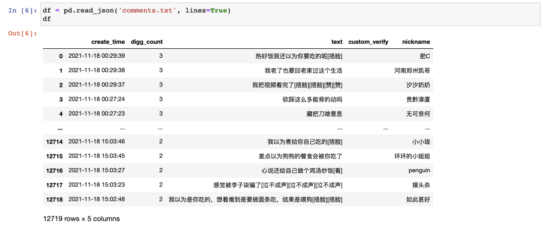
The text column is a comment.

First, do some exploratory analysis on the data. Several EDA tools have been introduced before, which can automatically produce basic data statistics and charts.

This time I use profile report

# eda
profile = ProfileReport(df, title='Tiktok's voice review data', explorative=True)
profile

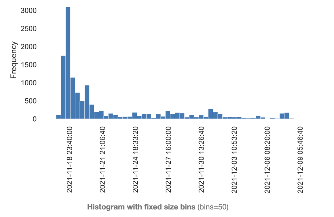
Comment time distribution

From the time distribution of comments, since the video was released on the 17th, there were a large number of comments on the 17th and 18th. However, in the future, even on December 9, there are still many new comments, indicating that the video is really hot.

Length distribution of comments

Most of the comments are within 20 words, basically no more than 40 words, and the explanations are short texts.

Reviewer identity

99.8% of the people who participated in the comments had no authentication, indicating that the comment users were basically ordinary users.

3. LDA

The above statistics are still too rough.

But if we want to know where everyone is interested, it is impossible to read all the 1.2w comments.

Therefore, these comments need to be classified first, which is equivalent to upgrading and abstracting the data. Because only by upgrading the data to dimension and understanding the meaning and proportion of each dimension can we master the data from a global perspective.

Here, I use LDA Algorithm to cluster texts, and the aggregated comments can be regarded as belonging to the same topic.

The core idea of LDA Algorithm has two points:

• Texts with certain similarities will aggregate together to form a theme. Each topic contains the words needed to generate the topic and the probability distribution of these words. In this way, the category of topics can be inferred artificially.

• Each article will have its probability distribution under all topics, so as to infer which topic the article belongs to.

For example, after clustering by LDA Algorithm, words such as war and military expenditure have a high probability in a topic, so we can classify the topic as military. If there is a high probability that an article belongs to a military topic, we can divide the article into military category.

After a brief introduction to the theory of LDA, let's practice it.

3.1 word segmentation and de stop words

#Participle

emoji = {'poor', 'In a daze', 'halo', 'suddenly have a brain wave', 'High five', 'Send heart', 'choke with sobs', 'Yawn', 'Lick the screen', 'Snicker', 'cheerful', 'bye', '666', 'Xiong Ji', 'Embarrassed smile', 'Spit out', 'Skimming', 'see', 'Green hat', 'facepalm ', 'Stay innocent', 'strong', 'shock', 'Insidious', 'most', 'Awesome', 'slap in the face', 'Coffee', 'decline', 'Let's come on together', 'Cool drag', 'shed tears', 'black face', 'love', 'Laugh and cry', 'witty', 'sleepy', 'Smiling kangaroo', 'strong', 'shut up', 'Come and see me', 'colour', 'Silly smile', 'A polite smile', 'Red face', 'Pick your nose', 'naughty', 'Crape myrtle, don't go', 'fabulous', 'Bixin', 'Leisurely', 'rose', 'Boxing', 'Little applause', 'handshake', 'Smirk', 'Shyness', 'I'm crying', 'Shh', 'surprised', 'pighead', 'spit', 'Observe secretly', 'Don't look', 'Beer', 'open the mouth and show the teeth', 'Get angry', 'A desperate stare', 'laugh', 'Hematemesis', 'Bad laugh', 'gaze', 'lovely', 'embrace', 'Wipe sweat', 'applause', 'victory', 'thank', 'reflection', 'smile', 'doubt', 'I want to be quiet', 'cognitive snap ', 'roll one's eyes', 'Tears running', 'yeah'}
stopwords = [line.strip() for line in open('stop_words.txt', encoding='UTF-8').readlines()]

def fen_ci(x):
    res = []
    for x in jieba.cut(x):
        if x in stopwords or x in emoji or x in ['[', ']']:
            continue
        res.append(x)
    return ' '.join(res)

df['text_wd'] = df['text'].apply(fen_ci)

Because there are many emoji expressions in the comments, I extracted the text corresponding to all emoji expressions and generated an emoji array to filter expression words.

3.2 calling LDA

from sklearn.feature_extraction.text import CountVectorizer
from sklearn.decomposition import LatentDirichletAllocation
import numpy as np

def run_lda(corpus, k):
    cntvec = CountVectorizer(min_df=2, token_pattern='\w+')
    cnttf = cntvec.fit_transform(corpus)
    
    lda = LatentDirichletAllocation(n_components=k)
    docres = lda.fit_transform(cnttf)
    
    return cntvec, cnttf, docres, lda
    
cntvec, cnttf, docres, lda = run_lda(df['text_wd'].values, 8)

After many tests, the data are divided into 8 categories, and the effect is good.

Select the words with top 20 probability under each topic:

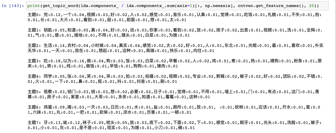
Distribution of subject words

From the probability distribution of these words, the categories of each topic are summarized. Topics 0 ~ 7 are: actually finished reading, knowing where the key is, rural life, feeding dogs, shooting techniques, locking the door Put more salt in eggs and socks under the pillow.

Proportion of statistical topics:

Subject proportion

Red is Theme 3 (feeding the dog), which accounts for the largest proportion. Many people commented that they thought they wanted to cook for themselves, but they didn't expect to feed the dog. I thought so when I saw it.

The proportion of other themes is relatively uniform.

After topic classification, we can find that Zhang not only attracted everyone's attention to rural life, but also a large number of abnormal scenes in the video.

Finally, the tree view is used to show each topic and the corresponding specific comments.

Articles under the theme

The picture is too large and only part of it is intercepted.

From grasping data to analysis, it was done in a hurry.

The core code has been posted in the article. The complete code is still being sorted out. If you need code or article, you can leave a message in the comment area.