Python learning -- the basic principle of principal component analysis (PCA) and its Python implementation

I. Basic Concept of dimensionality reduction

For the high-dimensional data in the actual analysis process, data dimensionality reduction processing is required before specific data analysis and feature modeling. Dimensionality reduction refers to selecting K (k < n) from the N features of the original data for data representation by some method, and realizing the compressed representation of the original data on the premise of reducing the loss of data information. Its main purposes include the following points:

(1) improve the utilization rate of data;

(2) reduce the computational overhead of the algorithm (software and hardware);

(3) remove interference noise;

(4) improve the interpretability of analysis results.

There are many existing data dimensionality reduction methods, According to personal understanding (insufficient understanding), according to the correlation between input variable X and target variable, it can be divided into input variable data dimensionality reduction (principal component analysis PCA, independent principal component analysis ICA, Factor Analysis FA, etc.) and correlation data dimensionality reduction (partial least squares PLS, Lasso, stepwise linear regression, regression number) (regression number can also be used for data dimensionality reduction), among the above methods, PCA is the most widely used and most widely spread. This time, only its basic principles and analysis ideas are introduced. Finally, through python programming, feel its great charm and finally analyze the limitations of the process.

II. PCA

In Mr. Zhou Zhihua's book machine learning, it is written that the greater the variance, the more information the data contains, which means that the more likely the changes between different samples and different dimensions of the data set can fully characterize the characteristics of the samples, and vice versa. What does this sentence mean? The greater the variance of a one-dimensional variable, the greater the amount of information it can contain, indicating that it has a greater 'voice' in the whole data. Generally speaking, the more knowledgeable and the wider the scope of knowledge, the more appropriate and clear the characteristics of all aspects of a thing. The main idea of PCA is based on the above principle, that is, by selecting K features (N) that can maximally measure and cover the original data, the dimension of data can be reduced, so as to improve the interpretability of the model and carry out visual analysis.

Before analyzing the basic principles of PCA, you need to understand the following concepts:

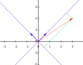
1. Geometric meaning of vector inner product

Hypothesis A,BIt is two non-zero vectors on a two-dimensional plane, and its inner product can be expressed as:

The coordinate axis is expressed as:

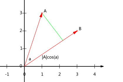
Among them,It actually represents the projection of vector A in the direction of vector B. When B is A unit vector, the inner product of A and B represents the projection of A vector on B vector and satisfies the above formula.

2. Transformation of basis

Base transformation is coordinate axis transformation (the main operation of PCA), which replaces the original coordinate axis by a new orthogonal axis (XOY coordinate axis). Here, the module of the base vector of the new coordinate axis must be 1 and orthogonal. The main reason is that the orthogonal matrix composed of two orthogonal unit vectors will not change the basic characteristic attributes (module, included angle and distance) of the vector when transforming the original coordinate axis orthogonally into the new coordinate axis. In addition, the basic characteristics of the orthogonal matrix()It is convenient for matrix reduction.

For vectors, assume that the new coordinate axis (Note: the base vector representation of the new coordinate axis is still based on the old coordinate axis) can be expressed as x axis respectivelyAnd y-axis. Then, according to the basic application of the inner product expressed in Section 1, the vector A on the new coordinate axis can be expressed as:

Among them,Is a matrix arranged by column vectors, that is, a transformation matrix;Is the coordinate representation under the new axis. The reason for right multiplication in the formula is that the transformation matrix is composed of column vectors, and each column represents a new coordinate axis. According to the calculation method of inner product, right multiplication is selected.

For example, for the vectors (3, 2) in the XOY coordinate system, suppose a new coordinate axis is selected, and its base vectors are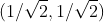and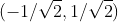, according to the meaning of the inner product expressed in the previous section, the expression of the vector on the new coordinate axis is:

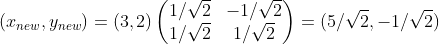
Specifically expressed as:

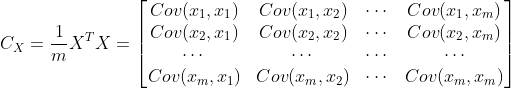
3. covariance matrix

As mentioned earlier, the greater the variance, the greater the amount of information. For the data shown in the figure below, the direction represented by XOY coordinates is not the direction with the largest variance. Combined with coordinate transformation, we can reconstruct a coordinate system (red line) based on the above concept, so that the sample information can be concentrated in a few coordinate axes as much as possible, and the remaining coordinate axes contain almost no information, which can be removed to realize feature dimension reduction.

The key problem now is how to measure the amount of information that can be represented by the coordinate axis. The first consideration is variance. For the transformed coordinates, assuming that the greater the variance of the data on a coordinate axis, the greater the amount of information contained in the data on that coordinate axis, In this way, we can select the required features (or coordinate axes) according to the size of variance for dimensionality reduction. However (most afraid of this), we have to consider a problem when doing data analysis, that is, the correlation of data.

Assuming that the axis with the largest variance is selected as the first dimension (the first transformation direction), when the correlation between variables is low or irrelevant, it can be considered to successively consider the corresponding axis with decreasing variance as the candidate transformation direction; however, when there is a strong correlation between the candidate first and second dimensions, that is, most of the information represented by the two are the same (the same here does not mean the size of the value, but the change of the represented sample characteristics, for example, with a simultaneous change trend). At this time, selecting the second dimension will not maximize the information representation, but will reduce the effective representation of the sample information. Therefore, other information consideration indicators need to be considered.

Covariance matrix represents whether two variables deviate from the mean at the same time. Diagonal variables represent the variance of each feature, and non diagonal variables represent the correlation between different features. The greater the absolute value, the stronger the correlation between variables. Covariance matrix combines the characteristics that the greater the variance, the greater the amount of information, and represents the correlation between different dimensions, so it can be used to measure the amount of variable information.

It is assumed that the input data after normalization is(normalization is used to reduce the interference of different value ranges of different dimensions), then its covariance matrix is:

Pseudo transformation matrix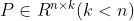, according to the matrix projectionDimensionality reduction from n-dimension to k-dimension can be realized. Where the covariance of Y matrix is:

According to the definition of matrix trace and covariance matrix, maximizing the retained data information is equivalent to the trace of maximizing covariance matrix, that is, the optimization objective can be expressed as:

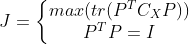
WhereRepresents the trace of the transformed coordinate covariance matrix,Is the constraint condition that the transformation matrix is orthogonal. According to Lagrange method, there are:

Because we used column vectors to represent samples, the derivation process here adopts denominator layout, including:

The following properties are used in the above formula:，.

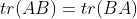Further, there are:

The properties used in the above formula are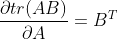, if the partial derivative expression is 0, there are:

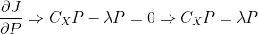
According to the definition of eigenvalue analysis, the final random result satisfies the relationship expression between eigenvector and eigenvalue, that is, byThe base matrix composed of the eigenvectors of the matrix is the obtained transformation matrix P. According to the basic meaning of feature transformation (eigenvalue)Representation matrixAbility to convert matrixIn the process of data dimensionality reduction, the basis vector with the largest information storage capacity must be the eigenvector corresponding to the maximum eigenvalue of the input matrix X covariance matrix, Therefore, we can solve the eigenvalue of the covariance matrix of the input matrix X, and select the corresponding transformation vector according to the absolute value of the eigenvalue, so as to realize the data dimensionality reduction.

So far, we have introduced the basic processing process and analysis principle of PCA, which is briefly described as follows:

step1: input matrix normalization;

Step 2: calculate the sample covariance matrix;

step3: solve the eigenvector corresponding to the specified number of maximum eigenvalues of the covariance matrix;

Step 4: determine the transformation matrix and solve the dimension reduction data.

III. PCA analysis by Python Programming

Based on the above steps, we successively carry out sub function programming (I like matlab, many expressions are not accurate in python, please understand), including:

#/usr/nom/env python
# _*_coding:utf-8_*_
# @Time      :2021/9/3 10:04
# @Author    :A bigfish
# @FileName  :maindemo13.py
# @Software  :PyCharm

import matplotlib.pyplot as plt
import numpy as np
from pylab import *

# First, import the data. This part reads the analysis data from the storage list or cell
def loadDataSet(filename, delim='\t'):    #'\ t' here represents the separator between different variables, and T represents the space typed by tab key
    fr = open(filename)
    stringArr = [line.strip().split(delim) for line in fr.readlines()]
    dataArr = [list(map(float, line)) for line in stringArr]
    return np.mat(dataArr)


# Define pca analysis function
def pca(dataset, topNfeat = 99999):        #The maximum number of topNfeat eigenvalues is usually not set because visual analysis is required later                
    meanVals = np.mean(dataset, axis=0)    #Find the mean
    meanRemoved = dataset - meanVals       #Pretreatment
    covMat = np.cov(meanRemoved, rowvar=0) #Solving the covariance matrix of input data
    eigVals, eigVects = np.linalg.eig(np.mat(covMat))    #Solving eigenvalues, eigenvectors
    eigVaInd = np.argsort(eigVals)         #Sort the characteristic values. The default value is ascending
    eigVaInd = eigVaInd[-1:-(topNfeat):-1] #Reverse the order according to the specified number
    redEigVects = eigVects[:,eigVaInd]     #Select the corresponding eigenvector
    lowDataMat = meanRemoved * redEigVects #Data dimensionality reduction X*P
    recontMat = (lowDataMat * redEigVects.T) + meanVals #c processing is used for data reconstruction, which is not a necessary option
    return lowDataMat, recontMat, eigVals  #Return data

# Define special value drawing function
def plotEig(dataset, numFeat=20):            
    mpl.rcParams['font.sans-serif'] = ['Times NewRoman']
    sumData = np.zeros((1, numFeat))
    dataset = dataset / sum(dataset)
    for i in range(numFeat):
        sumData[0, i] = sum(dataset[0:i])

    X = np.linspace(1, numFeat, numFeat)
    fig = plt.figure()
    ax = fig.add_subplot(211)
    ax.plot(X, (sumData*100).T, 'r-+')
    mpl.rcParams['font.sans-serif'] = ['SimHei']
    plt.ylabel('Cumulative variance percentage')

    ax2 = fig.add_subplot(212)
    ax2.plot(X.T, (dataset[0:numFeat].T)*100, 'b-*')
    plt.xlabel('Principal component fraction')
    plt.ylabel('Percentage variance')
    plt.show()

# Define the raw data and the first principal component drawing function
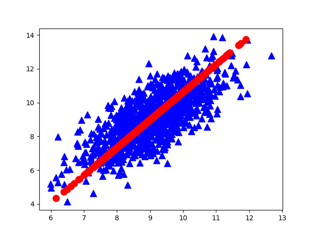
def plotData(OrigData, recData):
    import matplotlib.pyplot as plt
    fig = plt.figure()
    ax = fig.add_subplot(111)
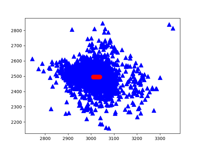
    ax.scatter(OrigData[:,0].flatten().A[0], OrigData[:, 1].flatten().A[0], c='blue',marker='^', s=90)
    ax.scatter(recData[:, 0].flatten().A[0], recData[:, 1].flatten().A[0], c='red', marker='o',s=90)
    plt.show()

In the main window buckle, there are:

if __name__ == '__main__':
    import maindemo13
    dataMat = maindemo13.loadDataSet('secom.txt', ' ') 
    newData = maindemo13.replaceNan(dataMat)    #This part is the missing value Nan processing function, which is not analyzed above
    lowData, recData, eigVals = maindemo13.pca(dataMat, 50)    #Select the first 50 features
    maindemo13.plotData(dataMat, recData)    #Draw the original data and the first principal component direction
    maindemo13.plotEig(eigVals, 50)    #Cumulative contribution rate of plotted eigenvalues

The obtained raw data (blue) and the first principal component analysis direction (red) are as follows:

The ranked principal component variance percentage and cumulative variance percentage are obtained

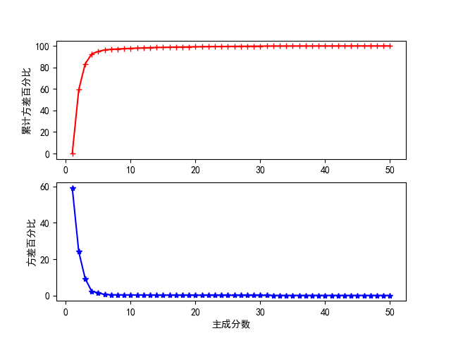
According to the variance percentage and cumulative variance of each principal component in the figure above, an appropriate principal component score can be selected for test analysis, but the best principal component score needs to be determined after cross validation.

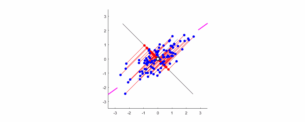
Finally, show me the dynamic diagram of pca analysis process drawn by myself with matlab, which is very good-looking!