1, Introduction to particle swarm optimization

1 concept of particle swarm optimization
Particle swarm optimization (PSO) is an evolutionary computing technology, which originates from the research on the predation behavior of birds. The basic idea of particle swarm optimization algorithm is to find the optimal solution through the cooperation and information sharing among individuals in the population
The advantage of PSO is that it is simple and easy to implement, and there is no adjustment of many parameters. At present, it has been widely used in function optimization, neural network training, fuzzy system control and other application fields of genetic algorithm.

2 particle swarm optimization analysis
2.1 basic ideas
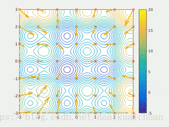
Particle swarm optimization algorithm designs a massless particle to simulate the birds in the bird swarm. The particle has only two attributes: speed and position. Speed represents the speed of movement and position represents the direction of movement. Each particle separately searches for the optimal solution in the search space, records it as the current individual extreme value, shares the individual extreme value with other particles in the whole particle swarm, and finds the optimal individual extreme value as the current global optimal solution of the whole particle swarm, All particles in the particle swarm adjust their speed and position according to the current individual extreme value found by themselves and the current global optimal solution shared by the whole particle swarm. The following dynamic diagram vividly shows the process of PSO algorithm:

2 update rules
PSO is initialized as a group of random particles (random solutions). Then the optimal solution is found by iteration. In each iteration, the particles update themselves by tracking two "extreme values" (pbest, gbest). After finding these two optimal values, the particle updates its speed and position through the following formula.

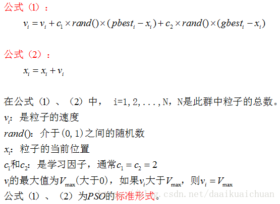
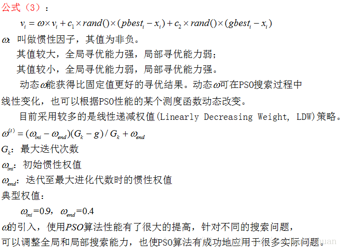
The first part of formula (1) is called [memory item], which indicates the influence of the last speed and direction; the second part of formula (1) is called [self cognition item], which is a vector from the current point to the best point of the particle itself, which indicates that the action of the particle comes from its own experience; the third part of formula (1) is called [group cognition item] is a vector from the current point to the best point of the population, which reflects the cooperation and knowledge sharing among particles. Particles determine the next movement through their own experience and the best experience of their peers. Based on the above two formulas, it forms the standard form of PSO.

Equations (2) and (3) are considered as standard PSO algorithms.
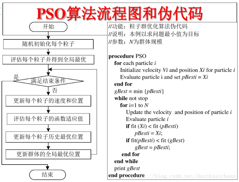
3 PSO algorithm flow and pseudo code

2, Partial source code

%%  optimization   +  PSO Solving location_Path optimization problem
%% Time: April 13, 2021:12:09
clc;clear;close all;
%% Initialize population
N = 300;                         % Number of initial population
d = 6;                           % Spatial dimension
ger =60;                         % Maximum number of iterations     
limit =zeros(2,2);
limit(:,1)=[-46000  63000 ];  
limit(:,2)=[-26000  70000 ] ;      
% Set position parameter limits
vlimit(1) = -10000;               % Set speed limit
vlimit(2)=10000 ;
wmax = 0.8;
wmin = 0.4;                        % Inertia weight
c1 = 1;                            % Self learning factor
c2 = 2;                            % Group learning factor 

model=CreateModel();               %Call model function
for i = 1:d
  if mod(i,2)==0
      x(:,i) = limit(2,1) + (limit(2,2) - limit(2,1)) * rand(N, 1);%Location of initial population
  else
      x(:,i) = limit(1,1) + (limit(1,2) - limit(1,1)) * rand(N, 1); 
  end
end
v = rand(N, d);                  % Speed of initial population
xm = x;                          % Historical best location for each individual
ym = zeros(1, d);                % Historical best position of population
fxm = 1./zeros(N,1);             % Historical best fitness of each individual
fym = inf;                       % Best fitness of population history   inf Infinity
%% Group renewal
iter = 1;
record = zeros(ger, 2);          % Recorder
average=record;
while iter <= ger
    fx=zeros(N,1);
    for i=1:N 
    fx(i)= TourLength(model,x(i,:)) ; % Individual current fitness   
    end
    intermediate_x=zeros(size(xm));
    intermediate_x(1:N,:) = xm;
    intermediate_x(N + 1 : N + N,1 : d) =  x;

  for i=1:N*2
     intermediate_x(i,d+3)=150;
     intermediate_x(i,d+1:d+2)=Tour(model, intermediate_x(i,:)) ; % Individual current fitness   
  end
    intermediate_x = ...
        non_domination_sort_mod(intermediate_x, 2, d);
    intermediate_x = replace_x(intermediate_x, 2, d, N);

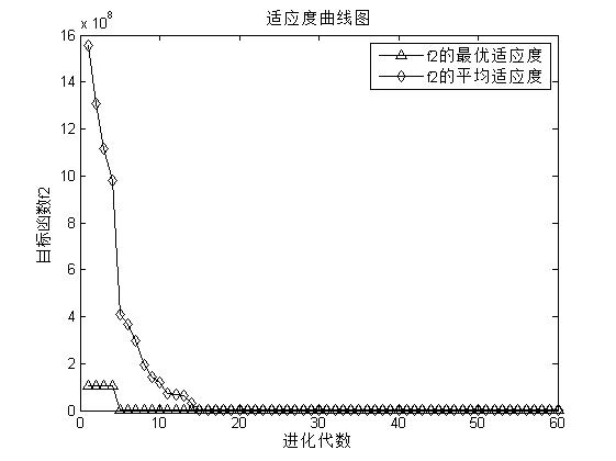
    record(iter,:) = intermediate_x(1,d+1:d+2);%Minimum mark
    average(iter,1)=sum(intermediate_x(:,d+1))/N;
    average(iter,2)=sum(intermediate_x(:,d+2))/N;
    ym=intermediate_x(1,1:d);
    fym=record(iter,:);
    
    disp(['The first',num2str(iter),'Second iteration''Minimum:',num2str(record(iter,:)),'Coordinates of emergency repair center:',num2str(ym)]);
    iter = iter+1;
    xm=intermediate_x(:,1:d);
    
    w=wmax-(wmax-wmin)*(ger-iter)/ger  ;%Weight update
    v = v * w + c1 * rand * (xm - x) + c2 * rand * (repmat(ym, N, 1) - x);% Speed update
    % Boundary velocity processing
    for ii=1:N
        for jj=1:d       
     if v(ii,jj)>vlimit(2)  v(ii,jj)= vlimit(2);end
      if v(ii,jj)<vlimit(1)  v(ii,jj)= vlimit(1);end
        end
    end
    x = x + v;% Location update
    % Boundary location processing
        for ii=1:N
        for jj=1:d         
             if mod(jj,2)==0 
                 if x(ii,jj)>limit(2,2)  x(ii,jj)= limit(2,2);end
                   if x(ii,jj)<limit(2,1)  x(ii,jj)= limit(2,1);end
             else
             if  x(ii,jj)>limit(1,2)  x(ii,jj)= limit(1,2);end
              if x(ii,jj)<limit(1,1)  x(ii,jj)= limit(1,1);end
             end
        end
        end
end

Schedule = code(x, model);  %call
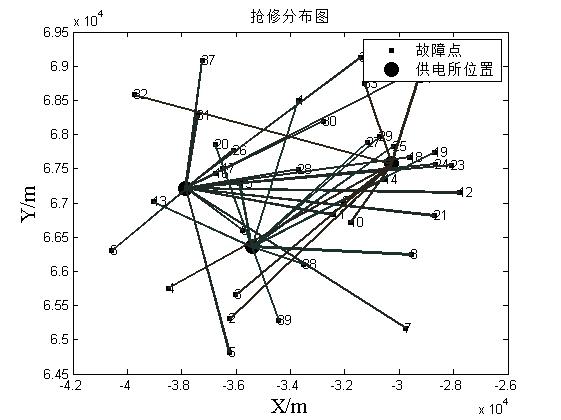
%% Plot test results
% Fault point
    figure(1);
    x=model.trouble(1,:);
    y=model.trouble(2,:);
    for i=1:39
        xx=x(i);
        yy=y(i);
        [ch1]=plot( xx,yy,'ks',...
           'MarkerFaceColor','k',...
           'MarkerSize',4); hold on
       text(xx , yy, num2str(i) );   %Dimensions with arrows
       hold on
    end
% Drawing emergency repair center
for i=1:3
    xx=ym(i*2-1);
    yy=ym(i*2);
    [ch2]= plot( xx ,yy ,'ko',...
        'MarkerFaceColor','k',...
        'LineWidth',6);hold on
    text(xx , yy, num2str( i) );   %Dimensions with arrows
    hold on
end

 %% Planning results
 rand('seed',  0);
 C= unifrnd(  0.1, 0.2,  model.Num_CenterSletectd , 3) ;%unifrnd You can create random, continuous, evenly distributed arrays
for i = 1: model.Num_CenterSletectd
     Center = Schedule(i).Center;
     Client =  Schedule(i).Client ;
     xx=model.trouble(1,:);
     yy=model.trouble(2,:);
    for j= Client
        x = [ ym(i*2-1) , xx(j ) ] ;
        y = [ ym(i*2)   , yy(j ) ] ;
 plot(   x ,y , '-' ,'color' ,C(i, : ) , 'linewidth' , 1.5 );  
    hold on
    end
end

% tagging
legend([ch1, ch2], {'Fault point'  ,'Location of power supply station' }); %  'Location','SouthWestOutside'Annotation placement
xlabel('X/m','fontsize',15,'fontname','Times new roman');
ylabel('Y/m','fontsize',15,'fontname','Times new roman');
title('Emergency repair distribution map'); 
axis on
set(gcf,'color',[1 1 1]);  %Set background color
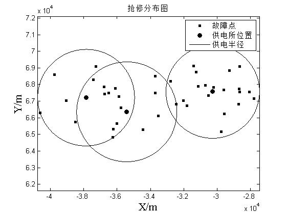
%% Draw power supply radius diagram
figure(2);
plot(model.trouble(1, : ), model.trouble(2, : ),'ks',...
      'MarkerFaceColor','k',...
      'MarkerSize',3);hold on
for i=1:3
    plot(ym(i*2-1),ym(i*2),'ko',...
        'MarkerFaceColor','k',...
        'MarkerSize',6);hold on    %  Distribution map of emergency repair center, radius
    x=ym(i*2-1);
    y=ym(i*2);
    r=model.point(3,i)*1000;
    theta=0:2*pi/3600:2*pi;
    Circle1=x+r*cos(theta);
    Circle2=y+r*sin(theta);
    plot(Circle1,Circle2,'k-','Linewidth',1);
    axis equal
end
legend('Fault point'  ,'Location of power supply station', 'Power supply radius');
title('Emergency repair distribution map');
xlabel('X/m','fontsize',15,'fontname','Times new roman');
ylabel('Y/m','fontsize',15,'fontname','Times new roman');

   for i=1:N 
      xm(i,d+1:d+2)=Tour(model,xm(i,1:d)) ; % Individual current fitness   
   end
   xm = non_domination_sort_mod(xm, 2, d);
 function f  = replace_chromosome(intermediate_chromosome, M, V,pop)


[N, m] = size(intermediate_chromosome);

% Get the index for the population sort based on the rank
[temp,index] = sort(intermediate_chromosome(:,M + V + 1));

clear temp m

% Now sort the individuals based on the index
for i = 1 : N
    sorted_chromosome(i,:) = intermediate_chromosome(index(i),:);
end

% Find the maximum rank in the current population
max_rank = max(intermediate_chromosome(:,M + V + 1));

% Start adding each front based on rank and crowing distance until the
% whole population is filled.
previous_index = 0;
for i = 1 : max_rank
    % Get the index for current rank i.e the last the last element in the
    % sorted_chromosome with rank i. 
    current_index = max(find(sorted_chromosome(:,M + V + 1) == i));
    % Check to see if the population is filled if all the individuals with
    % rank i is added to the population. 
    if current_index > pop
        % If so then find the number of individuals with in with current
        % rank i.
        remaining = pop - previous_index;
        % Get information about the individuals in the current rank i.
        temp_pop = ...
            sorted_chromosome(previous_index + 1 : current_index, :);
        % Sort the individuals with rank i in the descending order based on
        % the crowding distance.
        [temp_sort,temp_sort_index] = ...
            sort(temp_pop(:, M + V + 2),'descend');
        % Start filling individuals into the population in descending order
        % until the population is filled.
        for j = 1 : remaining
            f(previous_index + j,:) = temp_pop(temp_sort_index(j),:);
        end
        return;
    elseif current_index < pop
        % Add all the individuals with rank i into the population.
        f(previous_index + 1 : current_index, :) = ...
            sorted_chromosome(previous_index + 1 : current_index, :);
    else
        % Add all the individuals with rank i into the population.
        f(previous_index + 1 : current_index, :) = ...
            sorted_chromosome(previous_index + 1 : current_index, :);
        return;
    end

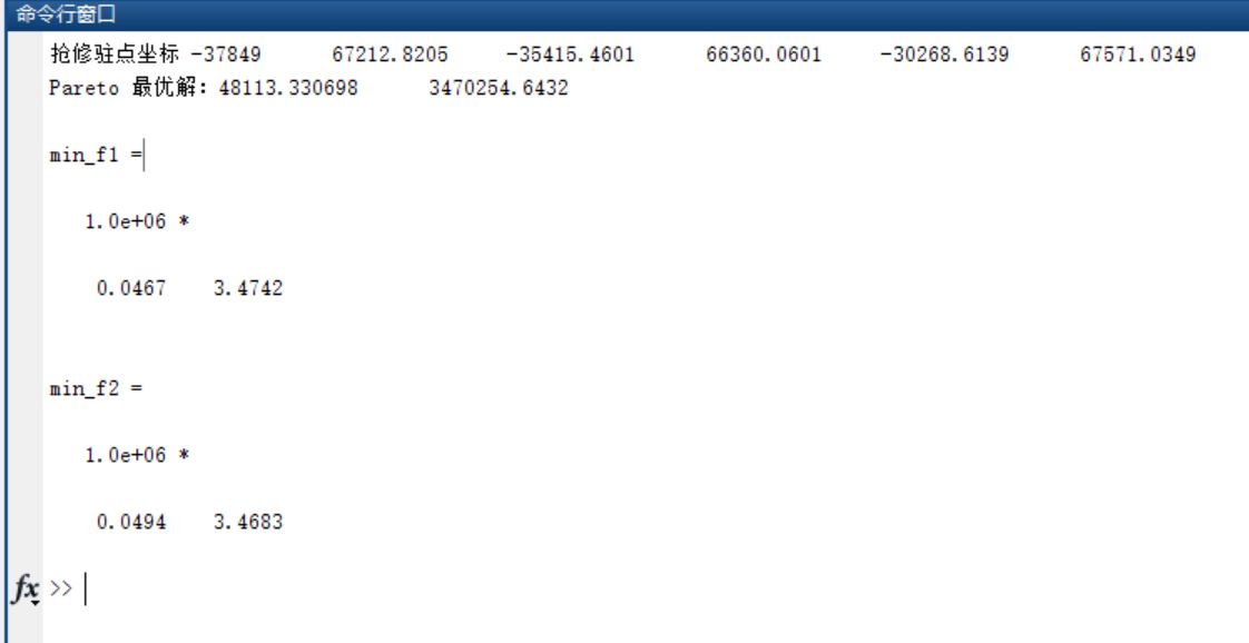
3, Operation results

4, matlab version and references

1 matlab version
2014a

2 references
[1] Steamed stuffed bun Yang, Yu Jizhou, Yang Shan Intelligent optimization algorithm and its MATLAB example (2nd Edition) [M]. Electronic Industry Press, 2016
[2] Zhang Yan, Wu Shuigen MATLAB optimization algorithm source code [M] Tsinghua University Press, 2017
[3] Zhou pin MATLAB neural network design and application [M] Tsinghua University Press, 2013
[4] Chen Ming MATLAB neural network principle and example refinement [M] Tsinghua University Press, 2013
[5] Fang Qingcheng MATLAB R2016a neural network design and application 28 case studies [M] Tsinghua University Press, 2018