1, Mathematical representation of fault information

In the figure above, K represents the circuit breaker, and each circuit breaker has an FTU device, which can feed back whether the circuit breaker switch is overcurrent, which represents the uploaded fault information, and reflects whether the fault current flows at each section switch (if there is fault current, it is 1, otherwise it is 0). Namely:

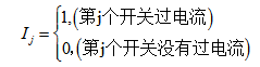
Because the information uploaded by FTU can be divided into fault information and no fault information, and it can only be fault and no fault for segmented interval, we can use binary coding rules to mathematically model the fault location problem of distribution network. Taking the radial distribution network shown in the figure above as an example, the system has 12 section switches. We can use a string of 12 bit binary code to represent the upload information of FTU as the input of the program. 1 represents that the corresponding switch has overcurrent information and 0 represents that the corresponding switch has no overcurrent information. At the same time, another string of 12 bit binary code is used as the output of the program to represent the failure of the corresponding feeder section and no failure.

The operation optimization of traditional distribution network mainly involves the adjustment of generator terminal voltage, the adjustment of transformer tap and the configuration of capacitor capacity. After the connection of distributed generation and energy storage devices, the optimization of distribution network will also include the control of distributed generation and energy storage devices. The objective function of distribution network operation optimization problem mainly includes minimizing the active power loss of the system, reducing the operation cost of equipment and so on. The optimization variables include continuous variables, i.e. the active and reactive power of distributed generation and energy storage device, discrete variables, i.e. the number of taps of transformer and switching groups of capacitor, the location and capacity of access equipment, etc. The main constraints are 1 Maximum and minimum limit of generator terminal voltage 2 Gear limit of transformer tap and capacity limit of capacitor 3 Limit of maximum daily operation number of transformers and capacitors, 4 Active and reactive power constraints of distributed generation and energy storage devices. Considering the objective function, variables and constraints of distribution network optimization, the optimization problem can be regarded as a multi-objective and multi variable mixed integer nonlinear programming problem.
At present, the main methods to solve the optimization problem of distribution network are traditional mathematical optimization method and artificial intelligence method. Traditional mathematical optimization methods mainly include linear / nonlinear programming method and dynamic programming method, while artificial intelligence methods mainly include genetic algorithm, simulated annealing method and particle swarm optimization algorithm. The traditional optimization algorithm considers the whole optimization problem from the overall situation, has strict principle and short calculation time. However, the initial values of objective function and optimization variables are highly required. Artificial intelligence algorithm has low requirements for objective function and initial value, and can solve high-dimensional optimization problems. Its disadvantage is easy to fall into local optimization and long calculation time.
To sum up, the main contents of the optimization direction of distribution network are: (1) research on the operation mode including distributed generation equipment and energy storage equipment (2) selection of installation location and capacity of distributed generation equipment and energy storage devices connected in distribution network (3) research on the optimization of operation and planning of distributed generation equipment and energy storage devices

2, Concept of particle swarm optimization

   particle swarm optimization (PSO) is an evolutionary computing technology. It originates from the research on the predation behavior of birds. The basic idea of particle swarm optimization algorithm is to find the optimal solution through the cooperation and information sharing among individuals in the population
   the advantage of PSO is that it is simple and easy to implement and there is no adjustment of many parameters. At present, it has been widely used in function optimization, neural network training, fuzzy system control and other application fields of genetic algorithm.

1. Basic thought

   particle swarm optimization algorithm simulates the birds in the bird swarm by designing a massless particle. The particle has only two attributes: speed and position. Speed represents the speed of movement and position represents the direction of movement. Each particle separately searches for the optimal solution in the search space, records it as the current individual extreme value, shares the individual extreme value with other particles in the whole particle swarm, and finds the optimal individual extreme value as the current global optimal solution of the whole particle swarm, All particles in the particle swarm adjust their speed and position according to the current individual extreme value found by themselves and the current global optimal solution shared by the whole particle swarm. The following dynamic diagram vividly shows the process of PSO algorithm:

2. Update rule

  PSO is initialized as a group of random particles (random solutions). Then the optimal solution is found by iteration. In each iteration, the particles update themselves by tracking two "extreme values" (pbest, gbest). After finding these two optimal values, the particle updates its speed and position through the following formula.

The first part of formula (1) is called [memory item], which indicates the influence of the last speed and direction; the second part of formula (1) is called [self cognition item], which is a vector from the current point to the best point of the particle itself, which indicates that the action of the particle comes from its own experience; the third part of formula (1) is called [group cognition item] is a vector from the current point to the best point of the population, which reflects the cooperation and knowledge sharing among particles. Particles determine the next movement through their own experience and the best experience of their peers. Based on the above two formulas, it forms the standard form of PSO.

%function main()
clear;
clc;
tic;
psoOptions = get_psoOptions; 
psoOptions.Vars.ErrGoal = 1e-6;     %Minimum error
LL=5;   %Number of tie switches
% Parameters common across all functions
psoOptions.SParams.c1 = 0.02; %Boundary parameters
psoOptions.SParams.w_beta = 0.5; %initialization beta value
 
% Run experiments for the three complex functions
psoOptions.Obj.f2eval = 'fitness_4geDG';
 
psoOptions.Obj.lb = ones(1,LL); %Initialization lower limit
%psoOptions.Obj.lb = ones(1,32);
psoOptions.Obj.ub = [10 7 15 21 11]; %Initialization upper limit            %By running the program maxswarmmin Results obtained
%psoOptions.Obj.ub = 20*ones(1,32);
%psoOptions.Obj.ub(1,1:5)=4;
psoOptions.SParams.Xmax =psoOptions.Obj.ub; %Maximum limit position
 
DimIters = [5; ...   %Dimensions dimension
              300];    %Corresponding iterations Number of iterations
  x = DimIters;        
psoOptions.Vars.Dim = x(1,:);
 psoOptions.Vars.Iterations = x(2,:);
 swarmsize = [50]   %Population size
psoOptions.Vars.SwarmSize = swarmsize;
disp(sprintf('This experiment will optimize %s function', psoOptions.Obj.f2eval));
disp(sprintf('Population Size: %d\t\tDimensions: %d.', psoOptions.Vars.SwarmSize, psoOptions.Vars.Dim));
temp = 5e6;
fVal = 0;
%function QPSO algorithm
 [tfxmin, xmin,PBest,fPBest, tHistory] = QPSO(psoOptions);
    fVal=tfxmin;
      if temp>tfxmin
        temp=tfxmin;
        record=tHistory;
      end
%%%%%%%%%%%%%%%%%%%%%%%%%%%%%%%%%%%%%%%%%%%%%%%%%%%%%%%%%%%%%%%%%%%%%%%%%%%%%%%%%%%%%%%%%%%%%%%%%%%%%%%%
toc;
disp(sprintf('\nminxfmin= \t\t%2.10g',temp));  %Optimal function fitness
xmin           %Optimized switch combination    
fPBest         %Adaptive value of alternative switch combination function
PBest          %Alternative switch combination(It is used to adopt alternative scheme in case of switch failure, which is more in line with the actual situation)
a=fbm(xmin)
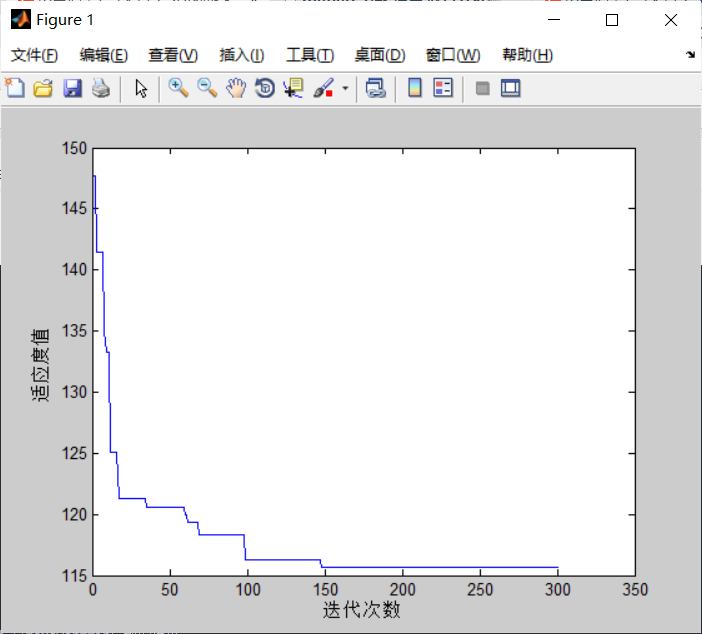
figure(1)
plot(record(:,2))
xlabel('Number of iterations')
ylabel('Fitness value')