Why dimensionality reduction?
reason
High dimensional machine learning has a large number of features (variables), which have certain obstacles to machine learning calculation, but some of them may have certain correlation. Under the condition of ensuring that there is no loss of too much information, the features are processed into a group of new variables to reduce the dimension to the original data.
Principal component analysis PAC
Principal component analysis (PAC) is the most widely used in dimension reduction.
thought
The dimension of the data set composed of a large number of related variables, while maintaining the variance of the data set as much as possible
Find a new set of variables. The original variables are just their linear combination
The new variable is called the Principal Component
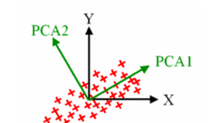
Understanding principles: Portal
Next, expand the PCA example using the built-in data set of iris
import pandas as pd
url = 'https://archive.ics.uci.edu/ml/machine-learning-databases/iris/iris.data'
df = pd.read_csv(url, names=['sepal length','sepal width','petal length','petal width','target'])
print(df.head())
The data is about this long

Step 1: Standardization
The StandardScaler method of the sklearn module is used here
from sklearn.preprocessing import StandardScaler
variables = ['sepal length','sepal width','petal length','petal width']
x = df.loc[:, variables].values
y = df.loc[:,['target']].values
x = StandardScaler().fit_transform(x)
x = pd.DataFrame(x)
print(x)
It looks like this after standardization
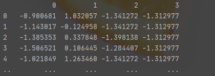
Step 2: PCA
from sklearn.decomposition import PCA
pca = PCA()
x_pca = pca.fit_transform(x)
x_pca = pd.DataFrame(x_pca)
x_pca.head()
It turned out like this
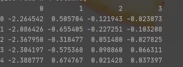
There are four characteristics in the original dataset. Therefore, PCA will provide the same number of principal components
We use PCA explained_ variance_ ratio_ To obtain the proportion of information extracted by each principal component
Step 3: calculate the principal component (variance contribution)
explained_variance = pca.explained_variance_ratio_
print(explained_variance)
# Returns a vector
[0.72770452 0.23030523 0.03683832 0.00515193]
Explanation: it shows that the first principal component accounts for 72.22% variance, and the second, third and fourth account for 23.9%, 3.68% and 0.51% variance. We can say that the first and second principal components capture 72.22 + 23.9 = 96.21% of the information. We often want to keep only important features and delete unimportant features. The rule of thumb is to retain the principal components that can capture significant variance and ignore the smaller variance.
Step 4: merge into new data
x_pca['target']=y
x_pca.columns = ['PC1','PC2','PC3','PC4','target']
x_pca.head()
Exhibition

Step 5: result visualization
import matplotlib.pyplot as plt
fig = plt.figure()
ax = fig.add_subplot(1,1,1)
ax.set_xlabel('Principal Component 1')
ax.set_ylabel('Principal Component 2')
ax.set_title('2 component PCA')
targets = ['Iris-setosa', 'Iris-versicolor', 'Iris-virginica']
colors = ['r', 'g', 'b']
for target, color in zip(targets,colors):
 indicesToKeep = x_pca['target'] == target
 ax.scatter(x_pca.loc[indicesToKeep, 'PC1']
 , x_pca.loc[indicesToKeep, 'PC2']
 , c = color
 , s = 50)
ax.legend(targets)
ax.grid()
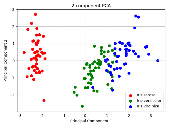
Surprisingly, principal component 12 is spatially separable.
Kernel PAC
In general, PAC is based on linear transformation, while KPAC is based on the results of nonlinear transformation, which is used to deal with linearly indivisible data sets.
The general idea of KPCA is: for the matrix [Formula] in the input space, we first map all the samples in the [Formula] to a high-dimensional or even infinite dimensional space (called Feature space) with a nonlinear mapping (make it linearly separable), and then reduce the dimension of PCA in this high-dimensional space.
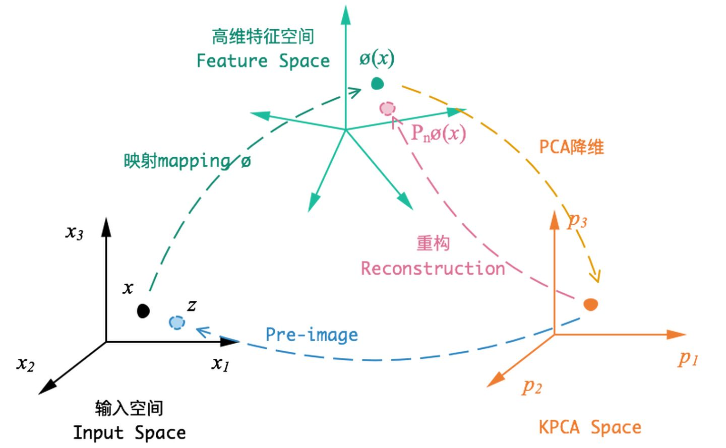
Principle analysis reference
Portal
Linear discriminant analysis LDA
Tip: the total number of learning plans is counted here
For example:
1. Technical notes 2 times
2. CSDN technology blog 3
3. 1 vlog video for learning