In any Automatic speech recognition system, the first step is to extract features. In other words, we need to extract the identifiable components from the audio signal, and then throw away other messy information, such as background noise, emotion and so on.

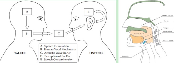
Understanding how speech is produced is very helpful for us to understand speech. People produce sound through the vocal tract, The shape of the channel determines what kind of sound is emitted. The shape of the channel includes the tongue, teeth, etc. if we can accurately know the shape, we can accurately describe the phoneme generated. The shape of the channel is displayed in the envelope of the speech short-term power spectrum. MFCCs is a feature that accurately describes the envelope.

MFCCs (Mel frequency cepstral coefficients) is a feature widely used in automatic speech and speaker recognition. It was developed by Davis and Mermelstein in 1980. Since then, in the field of speech recognition, MFCCs stands out among others in terms of artificial features and has never been surpassed (as for the feature learning of Deep Learning, that's later.).

Well, here we mention a very important keyword: the shape of the channel, and then know that it is very important, and that it can be displayed in the envelope of the speech short-term power spectrum. Hey, what is the power spectrum? What is envelope? What is MFCCs? Why does it work? How to get it? Let's talk slowly.

1, Spectrogram

We are dealing with voice signals, so how to describe it is very important. Because different descriptions show different information. So what kind of description is conducive to our observation and understanding? Here, let's first learn something called spectrogram.

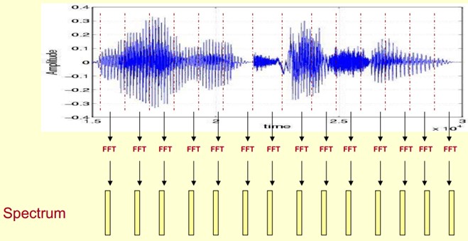
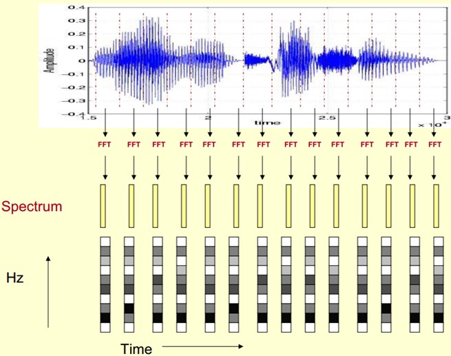
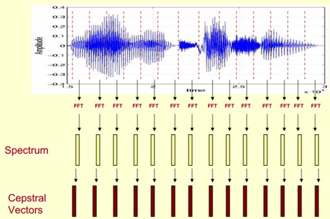
Here, the speech is divided into many frames, Each frame of speech corresponds to a spectrum (calculated by short-time FFT), which represents the relationship between frequency and energy. In practical use, there are three kinds of spectrum diagrams, namely linear amplitude spectrum, logarithmic amplitude spectrum and self power spectrum (the amplitude of each spectral line in logarithmic amplitude spectrum is logarithmically calculated, so the unit of ordinate is dB The purpose of this transformation is to make those components with low amplitude higher than those with high amplitude, so as to observe the periodic signal masked in low amplitude noise).

  

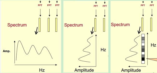
Let's first express the spectrum of one frame of speech through coordinates, as shown on the left in the figure above. Now let's rotate the spectrum on the left 90 degrees. Get the middle graph. These amplitudes are then mapped to a gray level representation (it can also be understood that the continuous amplitude is quantized into 256 quantized values?) 0 indicates black and 255 indicates white. The larger the amplitude value, the darker the corresponding area. In this way, the rightmost figure is obtained. Why? The dimension of time is added so that the spectrum of a speech can be displayed instead of a frame of speech, and the static and dynamic can be seen intuitively State information. The advantages will be presented later.

In this way, we will get a time-varying spectrum, which is the spectrogram of speech signal.

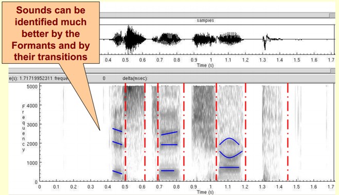
The following figure is the spectrogram of a speech. The dark place is the peak (formants) in the spectrogram.

So why do we represent speech in a spectrogram?

First, The properties of phonemes can be better observed here. In addition, the sound can be better recognized by observing formants and their transitions. Hidden Markov Models implicitly model the sound spectrum to achieve good recognition performance. Another function is that it can intuitively evaluate the TTS system The quality of (text to speech) can be directly compared with the matching degree of synthetic speech and natural speech spectrogram.

Through the time-frequency transformation of speech frames, the FFT spectrum of each frame is obtained, and then the spectrum of each frame is arranged in time order to obtain the time-frequency-energy distribution diagram. It intuitively shows the change of frequency center of speech signal with time.

2, Cepstrum Analysis

The following is a spectrum of speech. Peaks represent the main frequency components of speech. We call these peaks formants, and formants carry the recognition properties of sound (like personal ID card). Therefore, it is particularly important. It can recognize different sounds.

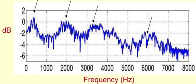
Since it is so important, we just need to extract it! We need to extract not only the positions of formants, but also their transformation process. So what we extract is the Spectral Envelope, which is a smooth curve connecting these formant points.

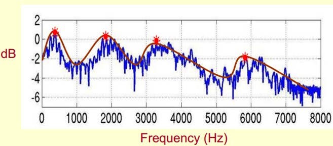
We can understand that the original spectrum consists of two parts: envelope and spectrum details. The logarithmic spectrum is used here, so the unit is dB. Now we need to separate the two parts so that we can get the envelope.

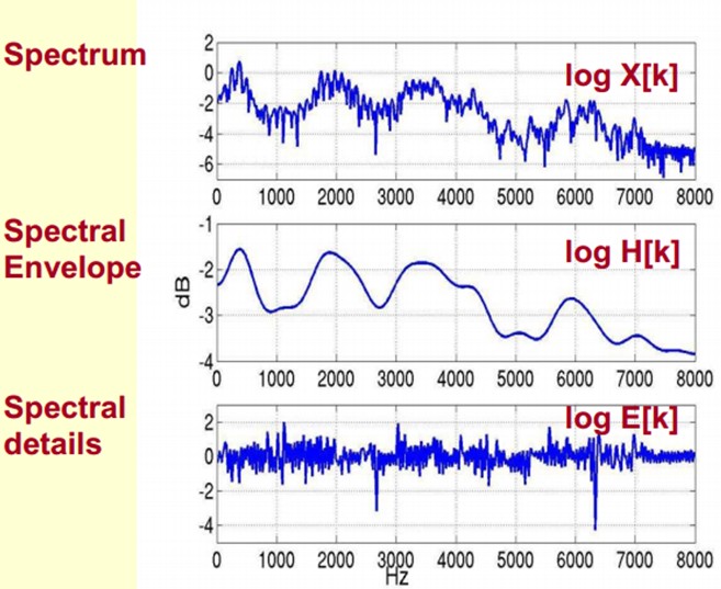
How do you separate them? That is, how to find log H[k] and log E[k] on the basis of given log X[k] to satisfy log X[k] = log H[k] + log E[k]?

To achieve this goal, we need to Play a Mathematical Trick. What is this Trick? Is to do FFT on the spectrum. Fourier transform in the spectrum is equivalent to inverse Fourier transform (IFFT). It should be noted that we deal with it in the logarithmic domain of the spectrum, which also belongs to Trick. At this time, doing IFFT on the logarithmic spectrum is equivalent to describing the signal on a pseudo frequency coordinate axis.

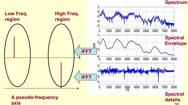
As we can see from the figure above, The envelope is mainly a low-frequency component (at this time, we need to change our thinking. At this time, the horizontal axis is not regarded as frequency, but as time). We regard it as a sinusoidal signal with 4 cycles per second. In this way, we give it a peak at 4Hz above the pseudo coordinate axis. The details of the spectrum are mainly high frequency. We regard it as a sinusoidal signal with 100 cycles per second. This So we give it a peak at 100Hz above the pseudo coordinate axis.

Put them together to make the original spectrum signal.

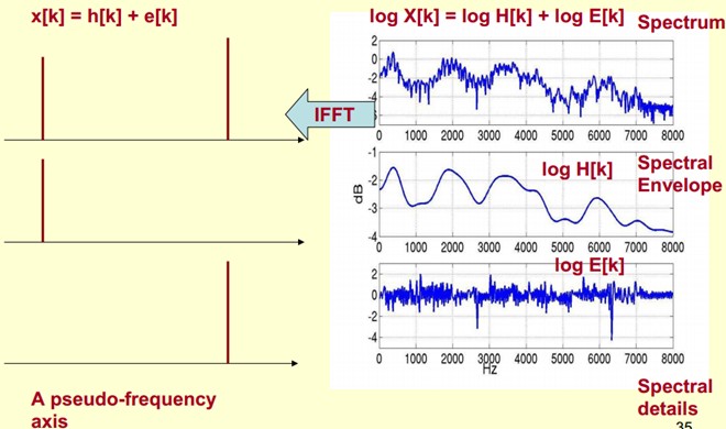
In practice, we already know log X[k], so we can get x[k]. Then we can know from the figure that h[k] is the low-frequency part of x[k], so we can get h[k] by passing x[k] through a low-pass filter! Yes, here we can separate them and get the h[k] we want, that is, the envelope of the spectrum.

x[k] is actually Cepstrum cepstrum (this is a newly created word, and the first four letters of spectrum word spectrum are inverted to be Cepstrum words). And we are concerned about h[k] is the low-frequency part of Cepstrum. h[k] describes the envelope of spectrum, which is widely used to describe features in speech recognition.

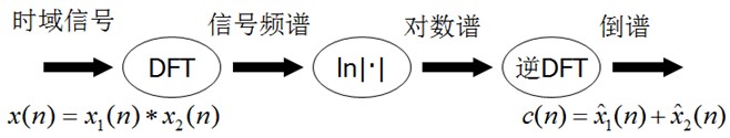
Now, to sum up, cepstrum analysis is actually such a process:

1) The spectrum of the original speech signal is obtained by Fourier transform: X[k]=H[k]E[k];

Consider only the amplitude: |x [k] | = | h [k] | E [k] |;

2) We take logarithms on both sides: log|x [k] | = log|h [k] | + log|e [k] |.

3) Then take the inverse Fourier transform on both sides to obtain: x[k]=h[k]+e[k].

This actually has a professional name called homomorphic signal processing. Its purpose is to transform nonlinear problems into linear problems. Corresponding to the above, The original speech signal is actually a rolling signal (the sound channel is equivalent to a linear time invariant system, and the generation of sound can be understood as an excitation through this system). In the first step, it is transformed into a multiplicative signal by convolution (the convolution in the time domain is equivalent to the product of the frequency domain). In the second step, the multiplicative signal is transformed into an additive signal by taking the logarithm, and in the third step, the inverse transform is performed to restore it to a curly signal. At this time, although the front and back are time-domain sequences, their discrete time domain is obviously different, so the latter is called cepstrum frequency domain.

In summary, cepstrum is the spectrum obtained by Fourier transform of a signal through logarithmic operation and then inverse Fourier transform. Its calculation process is as follows:

The following parts have not been sorted out

3, Mel frequency analysis

Well, here, let's see what we just did? Given a speech, we can get its spectral envelope (a smooth curve connecting all resonance peaks). However, the experiment of human auditory perception shows that human auditory perception only focuses on some specific areas, not the whole spectral envelope.

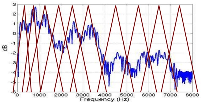
Mel frequency analysis is based on human auditory perception experiment. Experimental observations show that the human ear is like a filter bank, It only focuses on some specific frequency components (human hearing is selective to frequency). In other words, it only allows signals of certain frequencies to pass through, and directly ignores some frequency signals it doesn't want to perceive at all. However, these filters are not uniformly distributed on the frequency coordinate axis. There are many filters in the low-frequency region, which are densely distributed, but in the high-frequency region, the number of filters becomes smaller than that in the high-frequency region Less, very sparse distribution.

Human auditory system is a special nonlinear system. Its sensitivity to different frequency signals is different. In the extraction of speech features, the human auditory system does very well. It can extract not only semantic information, but also the speaker's personal features, which are beyond the reach of the existing speech recognition systems. If the human auditory perception processing characteristics can be simulated in the speech recognition system, it is possible to improve the speech recognition rate.

Mel frequency cepstrum coefficient (MFCC) takes into account the human auditory characteristics, first maps the linear spectrum to the Mel nonlinear spectrum based on auditory perception, and then converts it to cepstrum.

The formula for converting normal frequency to Mel frequency is:
 
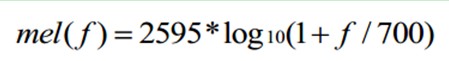
As can be seen from the figure below, it can convert non-uniform frequencies into uniform frequencies, that is, uniform filter banks.

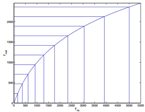
In Mel frequency domain, human perception of tone is linear. For example, if the Mel frequency of two speech segments is twice the difference, the human ear sounds that the two tones are twice the difference.

4, Mel frequency cepstral coefficients

We pass the spectrum through a set of Mel filters to obtain the Mel spectrum. The formula is: log X[k] = log (Mel spectrum). At this time, we perform cepstrum analysis on log X[k]:

1) log X[k] = log H[k] + log E[k].

2) Perform inverse transformation: x[k] = h[k] + e[k].

The cepstrum coefficient h[k] obtained on Mel spectrum is called Mel frequency cepstrum coefficient, or MFCC for short.

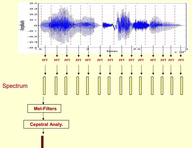
Now let's summarize the process of extracting MFCC features: (there are too many specific mathematical processes online, so I don't want to post them here)

1) Firstly, the speech is pre emphasized, divided into frames and windowed; (strengthen some preprocessing of speech signal performance (signal-to-noise ratio, processing accuracy, etc.)

2) For each short-time analysis window, the corresponding spectrum is obtained by FFT; (obtain the spectrum distributed in different time windows on the time axis)

3) The Mel spectrum is obtained by passing the above spectrum through the Mel filter bank; (convert the linear natural spectrum into Mel spectrum reflecting human auditory characteristics through Mel spectrum)

4) Carry out cepstrum analysis on Mel spectrum (take logarithm as inverse transform, and the actual inverse transform is generally realized through DCT discrete cosine transform. Take the second to 13th coefficients after DCT as MFCC coefficients) to obtain Mel frequency cepstrum coefficient MFCC, which is the feature of this frame; (cepstrum analysis, obtain MFCC as speech feature)

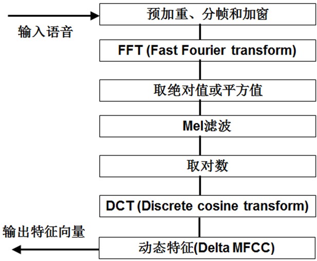
At this time, speech can be described by a series of cepstrum vectors, and each vector is the MFCC feature vector of each frame.

In this way, the speech classifier can be trained and recognized by these cepstrum vectors.

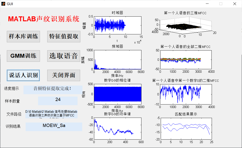
function varargout = GUI(varargin)
% GUI MATLAB code for GUI.fig
%      GUI, by itself, creates a new GUI or raises the existing
%      singleton*.
%
%      H = GUI returns the handle to a new GUI or the handle to
%      the existing singleton*.
%
%      GUI('CALLBACK',hObject,eventData,handles,...) calls the local
%      function named CALLBACK in GUI.M with the given input arguments.
%
%      GUI('Property','Value',...) creates a new GUI or raises the
%      existing singleton*.  Starting from the left, property value pairs are
%      applied to the GUI before GUI_OpeningFcn gets called.  An
%      unrecognized property name or invalid value makes property application
%      stop.  All inputs are passed to GUI_OpeningFcn via varargin.
%
%      *See GUI Options on GUIDE's Tools menu.  Choose "GUI allows only one
%      instance to run (singleton)".
%
% See also: GUIDE, GUIDATA, GUIHANDLES

% Edit the above text to modify the response to help GUI

% Last Modified by GUIDE v2.5 15-Mar-2020 17:37:45

% Begin initialization code - DO NOT EDIT
gui_Singleton = 1;
gui_State = struct('gui_Name',       mfilename, ...
                   'gui_Singleton',  gui_Singleton, ...
                   'gui_OpeningFcn', @GUI_OpeningFcn, ...
                   'gui_OutputFcn',  @GUI_OutputFcn, ...
                   'gui_LayoutFcn',  [] , ...
                   'gui_Callback',   []);
if nargin && ischar(varargin{1})
    gui_State.gui_Callback = str2func(varargin{1});
end

if nargout
    [varargout{1:nargout}] = gui_mainfcn(gui_State, varargin{:});
else
    gui_mainfcn(gui_State, varargin{:});
end
% End initialization code - DO NOT EDIT


% --- Executes just before GUI is made visible.
function GUI_OpeningFcn(hObject, eventdata, handles, varargin)
% This function has no output args, see OutputFcn.
% hObject    handle to figure
% eventdata  reserved - to be defined in a future version of MATLAB
% handles    structure with handles and user data (see GUIDATA)
% varargin   command line arguments to GUI (see VARARGIN)

% Choose default command line output for GUI
handles.output = hObject;

% Update handles structure
guidata(hObject, handles);

% UIWAIT makes GUI wait for user response (see UIRESUME)
% uiwait(handles.figure1);


% --- Outputs from this function are returned to the command line.
function varargout = GUI_OutputFcn(hObject, eventdata, handles) 
% varargout  cell array for returning output args (see VARARGOUT);
% hObject    handle to figure
% eventdata  reserved - to be defined in a future version of MATLAB
% handles    structure with handles and user data (see GUIDATA)

% Get default command line output from handles structure
varargout{1} = handles.output;


% --- Executes on button press in pushbutton1.
function pushbutton1_Callback(hObject, eventdata, handles)
fprintf('\n Identifying...\n\n');
%Load trained GMM Model
load speakerData;
load speakerGmm;

waveDir='trainning\';  %Import test set
Test_speakerData = dir(waveDir);   %Get the structure data in the test set. This is a char Structure of type
Test_speakerData(1:2) = [];
Test_speakerNum=length(Test_speakerData);
Test_speakerNum
count=0;
%%%%%%%%%%%%%%%%for i=1:Test_speakerNum
%%%Read voice
[filename,filepath]=uigetfile('*.wav','Select audio file');
set(handles.text1,'string',filepath)
   filep=strcat(filepath,filename); 
[testing_data, fs]=wavread(filep);
sound(testing_data, fs);
save testing_data
load testing_data
y=testing_data
axes(handles.axes1)
plot(y);
xlabel('t');ylabel('amplitude');
title('Time domain diagram');
%frequency domain
%Amplitude frequency diagram
N=length(y);   
fs1=100;  %sampling frequency 
n=0:N-1;
t=n/fs;   %time series
yfft =fft(y,N);
mag=abs(yfft);     %Take the absolute value of the amplitude
f=n*fs/N;    %Frequency sequence
axes(handles.axes2)
plot(f(1:N/2),mag(1:N/2)); %draw Nyquist Amplitude varying with frequency before frequency
xlabel('frequency/Hz');
ylabel('amplitude');title('Frequency domain diagram');

%Phase spectrum
A=abs(yfft);
ph=2*angle(yfft(1:N/2));
ph=ph*180/pi;
axes(handles.axes3);
plot(f(1:N/2),ph(1:N/2));
xlabel('frequency/hz'),ylabel('phase angle'),title('Number 0-9 Phase spectrum of');
% Draw power spectrum
Fs=1000;
n=0:1/Fs:1;
xn=y;
nfft=1024;
window=boxcar(length(n)); %Rectangular window
noverlap=0; %No data overlap
p=0.9; %Confidence probability
[Pxx,Pxxc]=psd(xn,nfft,Fs,window,noverlap,p);
index=0:round(nfft/2-1);
k=index*Fs/nfft;
plot_Pxx=10*log10(Pxx(index+1));
plot_Pxxc=10*log10(Pxxc(index+1));
axes(handles.axes4)
plot(k,plot_Pxx);
title('Number 0-9 Power spectrum of');

axes(handles.axes5)
surf( speakerData(1).mfcc);  %draw MFCC 3D drawing of
title('Three dimensional of the first person's voice MFCC');   %The first person to speak mfcc Characteristics of   mfcc It refers to Mel cepstrum coefficient

%Draw the first person's MFCC All 2D drawings of
axes(handles.axes6)

plot(speakerData(1).mfcc);
title('All two dimensions of the first person's voice MFCC');

%To see the effect, draw a feature
axes(handles.axes7)
plot(speakerData(1).mfcc(:,2));
title('Two dimensional of the first digit 0 in the first person's voice MFCC');


% hObject    handle to pushbutton1 (see GCBO)
% eventdata  reserved - to be defined in a future version of MATLAB
% handles    structure with handles and user data (see GUIDATA)


% --- Executes on button press in pushbutton2.
function pushbutton2_Callback(hObject, eventdata, handles)
load testing_data
load speakerGmm
match= MFCC_feature_compare(testing_data,speakerGmm);
axes(handles.axes8)
plot(match);
hold on
title('Display of matching results');
[max_1 index]=max(match);
fprintf('\n %s',match);
fprintf('\n\n\n The speaker is%s. ',speakerData(index).name(1:end-4))
set(handles.text3,'string',speakerData(index).name(1:end-4))
if index==i
  count=count+1;
end


% hObject    handle to pushbutton2 (see GCBO)
% eventdata  reserved - to be defined in a future version of MATLAB
% handles    structure with handles and user data (see GUIDATA)


% --- Executes on button press in pushbutton3.
function pushbutton3_Callback(hObject, eventdata, handles)
waveDir = uigetdir(strcat(matlabroot,'\work'), 'Select training audio library' );
set(handles.text8,'string','Sample library selection completed!')
speakerData = dir(waveDir);  % Get the structure data in the test set. This is a char Structure of type
speakerData(1:2) = [];
speakerNum=length(speakerData);%Number of test personnel;
set(handles.text6,'string',speakerNum)
save speakerNum

% hObject    handle to pushbutton3 (see GCBO)
% eventdata  reserved - to be defined in a future version of MATLAB
% handles    structure with handles and user data (see GUIDATA)


% --- Executes on button press in pushbutton4.
function pushbutton4_Callback(hObject, eventdata, handles)
load speakerNum
set(handles.text8,'string','Audio file feature extraction in progress...')
pause(1) %Stay for one second
for i=1:speakerNum
	fprintf('\n Extracting page%d personal%s Characteristics of', i, speakerData(i,1).name(1:end-4));
       
    [y, fs]=wavread(['trainning\' speakerData(i,1).name]);  %Read the audio data of the sample
    y=double(y);    %Type conversion
    y=y/max(y);
    epInSampleIndex = epdByVol(y, fs);		% Endpoint detection
    y=y(epInSampleIndex(1):epInSampleIndex(2));	% Eliminate noise
    speakerData(i).mfcc=melcepst(y,8000);
end
 set(handles.text8,'string','Audio feature extraction is complete!')
 save speakerData speakerData		% Save data
% hObject    handle to pushbutton4 (see GCBO)
% eventdata  reserved - to be defined in a future version of MATLAB
% handles    structure with handles and user data (see GUIDATA)


% --- Executes on button press in pushbutton5.
function pushbutton5_Callback(hObject, eventdata, handles)
%GMM train
fprintf('\n Train each speaker's Gaussian mixture model...\n\n');
load speakerData.mat
gaussianNum=12;					
speakerNum=length(speakerData);  %Number of samples obtained


for i=1:speakerNum
	fprintf('\n For the first%d A speaker%s train GMM......', i,speakerData(i).name(1:end-4));
	[speakerGmm(i).mu, speakerGmm(i).sigm,speakerGmm(i).c] = gmm_estimate(speakerData(i).mfcc(:,5:12)',gaussianNum,20);  %Transpose correct
 
end

fprintf('\n');
save speakerGmm speakerGmm;   %Save sample GMM
% hObject    handle to pushbutton5 (see GCBO)
% eventdata  reserved - to be defined in a future version of MATLAB
% handles    structure with handles and user data (see GUIDATA)


% --- Executes on button press in pushbutton6.
function pushbutton6_Callback(hObject, eventdata, handles)
clc
close all
% hObject    handle to pushbutton6 (see GCBO)
% eventdata  reserved - to be defined in a future version of MATLAB
% handles    structure with handles and user data (see GUIDATA)