Note: This is a machine learning practical project (with data + code). If you need data + complete code, you can get it directly at the end of the article.

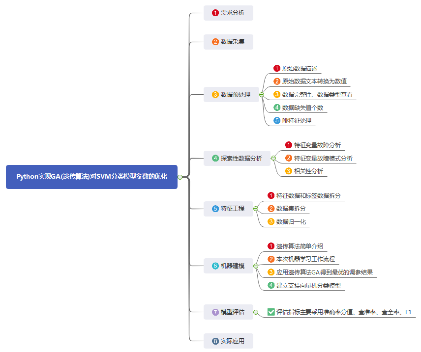
1. Demand analysis

In the environment of intensive introduction of a series of national policies and driven by strong demand in the domestic market, China's domestic gas stove industry as a whole has maintained steady and rapid growth. With the increase of industrial investment, technological breakthrough and scale accumulation, it begins to usher in an accelerated period of development in the foreseeable future. The sales of gas stove products of an electrical appliance company has always been in a leading position in China. It regards product quality as the top priority. It is necessary to analyze and study its product quality data every year in order to continuously improve and keep improving. This model is also based on some historical data to model and predict the maintenance mode.

2. Data acquisition

This data is analog data and is divided into two parts:

Dataset: data xlsx

In practical application, you can replace it according to your own data.

Characteristic data: failure mode, failure mode breakdown, failure name, and document type

Tag data: maintenance mode

3. Data preprocessing

1) Raw data description:

2) Convert raw data text to numeric values:

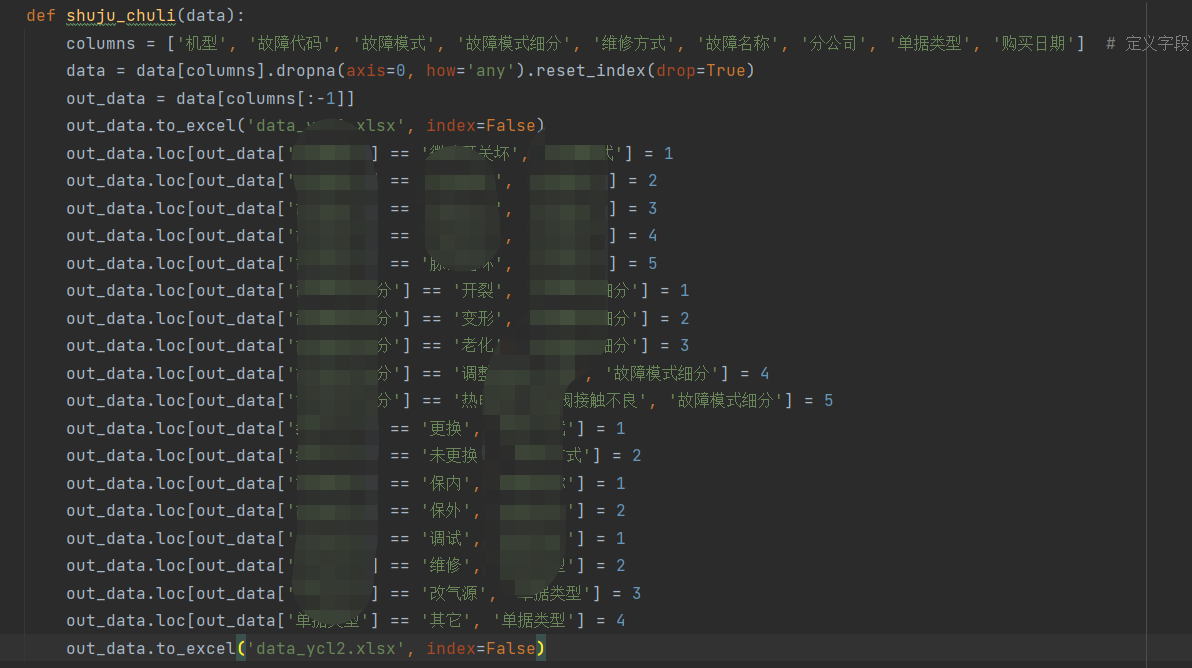
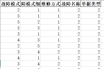
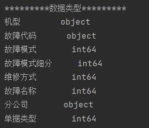
2) Data integrity and data type viewing:

print(data_.dtypes)  # Print data type

3) Number of missing data values:

print(data_.isnull().any())  # Check for NULL values

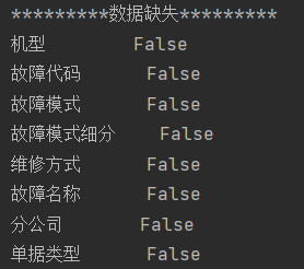
You can see that there are no missing values in the data.

4) Dumb feature processing

The values in the characteristic variable fault mode, fault mode subdivision and fault name are text types, which do not meet the requirements of machine learning data. Dummy feature processing is required and become 0.1 value.

The key codes are as follows:

After processing, the data are as follows:

 4. Exploratory data analysis

1) Characteristic variable fault analysis:

Fault analysis: in the maintenance records, the maintenance quantities of different parts are different, and the number of "electrode needle failure" accounts for the most, accounting for 64.12% of all maintenance records. "Thermocouple failure" and "solenoid valve failure" took the second place, 14.87% and 11.29% respectively.

explodes = [0.1 if i == "sales" else 0 for i in lbs]
matplotlib.rcParams['font.sans-serif'] = ['SimHei']
plt.figure(figsize=(5, 5))  # Create a subgraph with a size of 5 * 5
patches, l_text, p_text = plt.pie(data["Failure mode"].value_counts(normalize=True), explode=explodes,
                                  labels=lbs, autopct='%.2f%%', radius=0.8)
for t in p_text:
    t.set_size(12)
for t in l_text:
    t.set_size(12)
plt.show()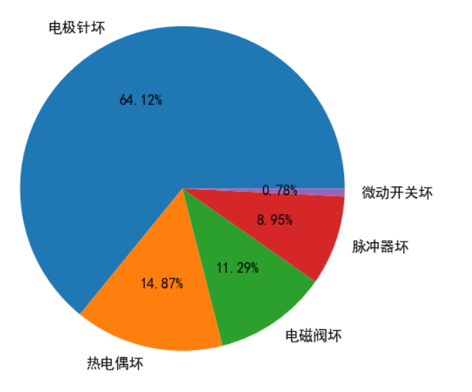

2) Characteristic variable failure mode analysis:

The failure modes are subdivided into 5 items: "cracking", "deformation", "aging", "adjusting the position of electrode needle" and "poor contact between thermocouple and solenoid valve".

def pie_pic(data, color=None, radius=None):
    lbs = data.value_counts().index
    if color:
        matplotlib.rcParams['font.sans-serif'] = ['SimHei']
        plt.pie(data.value_counts(normalize=True), labels=lbs, colors=sns.color_palette(color, 4),
                autopct='%.2f%%', radius=radius, startangle=120)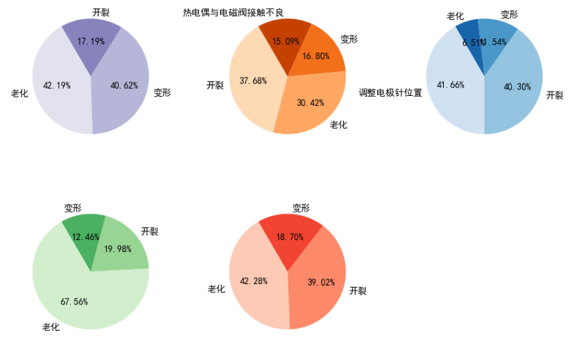

3) Correlation analysis

df_tmp1 = df_data[
    ['Failure mode_1', 'Failure mode_2', 'Failure mode_3', 'Failure mode_4', 'Failure mode_5', 'Fault mode subdivision_1', 'Fault mode subdivision_2', 'Fault mode subdivision_3', 'Fault mode subdivision_4', 'Fault mode subdivision_5',
     'Fault name_1', 'Fault name_2', 'Maintenance mode']]
plt.rcParams['font.sans-serif'] = ['SimHei']
plt.rcParams['axes.unicode_minus'] = False
sns.heatmap(df_tmp1.corr(), cmap="YlGnBu", annot=True)
plt.show()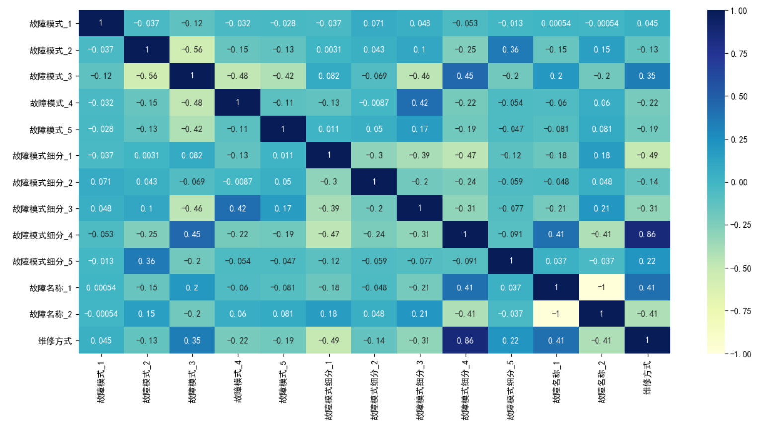

Note: when positive value is positive correlation and negative value is negative correlation, the greater the value, the stronger the correlation between variables.

5. Characteristic Engineering

1) The feature data and label data are split, y is label data, and those other than y are feature data;

2) The data set is divided into training set and trial set, 80% training set and 20% verification set;

3) Data normalization

6. Machine modeling

1) Brief introduction to genetic algorithm:

Genetic Algorithm, also known as Genetic Algorithm, is called GA algorithm for short. Since it is called Genetic Algorithm, there must be genes in heredity, and the gene chromosome is its parameter to be adjusted. We have learned in biology that the law of nature is "natural selection, survival of the fittest". I think Genetic Algorithm is more suitable for "survival of the fittest".

1. Excellent: optimal solution,
2. Inferior: non optimal solution.

Implementation process of genetic algorithm:

It also involves fitness function, selection, crossover and mutation. These modules are described below. The specific flow chart is explained as follows:

(1) It is necessary to calculate the fitness function of the initial population first, so as to facilitate us to select individuals. The larger the fitness value, the easier it is to be retained;

(2) Select the population and select a part of the dominant population with large fitness value;

(3) It is easier to produce excellent individuals by "mating" the dominant population;

(4) Simulate the natural mutation operation, and carry out mutation operation on chromosome individuals;

2) Workflow of this machine learning:

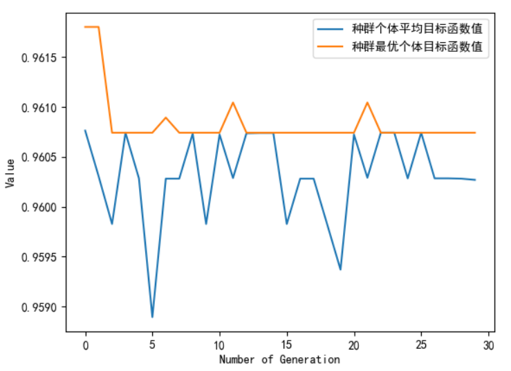
(1) The population number NIND = 50 represents that the first generation population first carries out 50 times of model training as 50 initial individuals, and the [C, G] of each training (of course, the C and G of each training are also randomly initialized) is the chromosome of this individual;

(2) The objective function is the classification accuracy on the training set (of course, the cross validation score used in the following code actually has the same meaning);

(3) Selection, crossover, variation, evolution

(4) Finally, the optimal individuals in the last generation population get the C and Gamma we want, and substitute these two parameters into the test set to calculate the test set results

3) Genetic algorithm GA is used to obtain the optimal parameter adjustment results

number	name
1	Number of evaluations: 750
2	2950.9299054145813 seconds have elapsed
3	The optimal objective function value is 0.9611955168119551
4	The optimal control variable value is:
5	Value of C: 149.7418557703495
6	Value of G: 0.00390625

The optimal values of null variables C and G can be tried slowly in the process of actual data set.

4) A support vector machine classification model is established. The model parameters are as follows:

number	parameter
1	C=C
2	kernel='rbf'
3	gamma=G

Other parameters are set according to specific data.

7. Model evaluation

1) The evaluation indicators mainly include accuracy score, precision, recall and F1

number	Evaluation index name	Evaluation index value
1	Accuracy score	0.96
2	Precision rate	95.02%
3	Recall	99.73%
4	F1	97.32%

It can be seen from the above table that the effect of this model is good.

class MyProblem(ea.Problem):  # Inherit Problem parent class
    def __init__(self, PoolType):  # PoolType is a string with a value of 'Process' or' Thread '
        name = 'MyProblem'  # Initialization name (function name, which can be set at will)
        M = 1  # Initialize M (target dimension)
        maxormins = [-1]  # Initialize maxormins (target min max tag list, 1: minimize the target; - 1: maximize the target)
        Dim = 2  # Initialize Dim (decision variable dimension)
        varTypes = [0, 0]  # Initialize varTypes (the type of the decision variable. If the element is 0, the corresponding variable is continuous; if 1, it is discrete)
        lb = [2 ** (-8)] * Dim  # Lower bound of decision variable
        ub = [2 ** 8] * Dim  # Upper bound of decision variable
        lbin = [1] * Dim  # Lower boundary of decision variable (0 means the lower boundary of the variable is not included, and 1 means the lower boundary of the variable is included)
        ubin = [1] * Dim  # Upper boundary of decision variable (0 means the upper boundary of the variable is not included, and 1 means included)
        # Call the parent class constructor to complete instantiation
        ea.Problem.__init__(self, name, M, maxormins, Dim, varTypes, lb, ub, lbin, ubin)
        # Some data used in objective function calculation

        ori_data = pd.read_excel("data.xlsx", header=1)
        print(ori_data.head())

        # Read preprocessed data

        self.data = preprocessing.scale(np.array(X_train))  # Characteristic data of training set (normalized)
        self.dataTarget = np.array(Y_train)
        # Set whether to use multithreading or multiprocessing
        self.PoolType = PoolType
        if self.PoolType == 'Thread':
            self.pool = ThreadPool(2)  # Set the size of the pool
        elif self.PoolType == 'Process':
            num_cores = int(mp.cpu_count())  # Get the number of cores of the computer
            self.pool = ProcessPool(num_cores)  # Set the size of the pool

    def aimFunc(self, pop):  # The objective function adopts multithreading to accelerate the calculation
        Vars = pop.Phen  # The decision variable matrix is obtained
        args = list(
            zip(list(range(pop.sizes)), [Vars] * pop.sizes, [self.data] * pop.sizes, [self.dataTarget] * pop.sizes))
        if self.PoolType == 'Thread':
            pop.ObjV = np.array(list(self.pool.map(subAimFunc, args)))
        elif self.PoolType == 'Process':
            result = self.pool.map_async(subAimFunc, args)
            result.wait()
            pop.ObjV = np.array(result.get())

    def test(self, C, G):  # Substitute the optimized C and Gamma to test the test set

        data_test = pd.read_excel("data_test.xlsx")
        X_test = data_test.drop(columns=['Maintenance mode'])
        Y_test = data_test['Maintenance mode']

        data_test = preprocessing.scale(np.array(X_test))  # Characteristic data of test set (normalized)
        dataTarget_test = np.array(Y_test)  # Label data for test set
        svc = svm.SVC(C=C, kernel='rbf', gamma=G).fit(self.data, self.dataTarget)  # Create a classifier object and fit the classifier model with the data of the training set
        dataTarget_predict = svc.predict(X_test)  # The trained classifier object is used to predict the test set data
        print("Test set data classification accuracy = %s%%" % (
                    len(np.where(dataTarget_predict == dataTarget_test)[0]) / len(dataTarget_test) * 100))
        print("Verification set precision: {:.2f}%".format(precision_score(Y_test, dataTarget_predict) * 100))  # Print verification set precision
        print("Verification set recall: {:.2f}%".format(recall_score(Y_test, dataTarget_predict) * 100))  # Print verification set recall
        print("Validation set F1 value: {:.2f}%".format(f1_score(Y_test, dataTarget_predict) * 100))  # Print validation set F1 value


def subAimFunc(args):
    i = args[0]
    Vars = args[1]
    data = args[2]
    dataTarget = args[3]
    C = Vars[i, 0]
    G = Vars[i, 1]
    svc = svm.SVC(C=C, kernel='rbf', gamma=G).fit(data, dataTarget)  # Create a classifier object and fit the classifier model with the data of the training set
    scores = cross_val_score(svc, data, dataTarget, cv=30)  # Calculate the score of cross validation
    ObjV_i = [scores.mean()]  # Take the average score of cross validation as the objective function value
    return ObjV_i

import geatpy as ea  # import geatpy

if __name__ == '__main__':
    """===============================Instantiate problem object==========================="""
    PoolType = 'Thread'  # The setting adopts multithreading. If it is modified to PoolType = 'Process', it means multithreading
    problem = MyProblem(PoolType)  # Generate problem object
    """=================================Population setting=============================="""
    Encoding = 'RI'  # Coding mode
    NIND = 50  # Population size
    Field = ea.crtfld(Encoding, problem.varTypes, problem.ranges, problem.borders)  # Create area descriptor
    population = ea.Population(Encoding, Field, NIND)  # Instantiate the population object (at this time, the population has not been initialized, but only the instantiation of the population object is completed)
    """===============================Algorithm parameter setting============================="""
    myAlgorithm = ea.soea_SGA_templet(problem, population)
    myAlgorithm.MAXGEN = 30  # Maximum algebra
    myAlgorithm.trappedValue = 1e-6  # "Evolution stagnation" judgment threshold
    myAlgorithm.maxTrappedCount = 10  # The maximum upper limit of the evolution stagnation counter. If the continuous maxTrappedCount generation is judged that the evolution is stagnant, the evolution will be terminated
    myAlgorithm.logTras = 1  # Set how many generations of logs are recorded. If it is set to 0, it means that logs are not recorded
    myAlgorithm.verbose = True  # Set whether to print log information
    myAlgorithm.drawing = 1  # Set the drawing method (0: do not draw; 1: draw the result diagram; 2: draw the target space process animation; 3: draw the decision space process animation)
    """==========================Call the algorithm template for population evolution========================"""
    [BestIndi, population] = myAlgorithm.run()  # Execute the algorithm template to obtain the optimal individual and the last generation population
    BestIndi.save()  # Save the information of the optimal individual to a file
    """=================================Output results=============================="""
    print('Evaluation times:%s' % myAlgorithm.evalsNum)
    print('Time has passed %s second' % myAlgorithm.passTime)
    if BestIndi.sizes != 0:
        print('The optimal objective function value is:%s' % (BestIndi.ObjV[0][0]))
        print('The optimal control variable value is:')
        for i in range(BestIndi.Phen.shape[1]):
            print(BestIndi.Phen[0, i])
        """=================================Inspection results==============================="""
        problem.test(C=BestIndi.Phen[0, 0], G=BestIndi.Phen[0, 1])
    else:
        print('No feasible solution was found.')

8. Practical application

According to the characteristic data of the test set, the maintenance mode of these products is predicted. Product optimization and personnel work arrangement can be carried out according to the predicted maintenance mode type. The specific prediction results are not pasted here.

The project resources are as follows: https://download.csdn.net/download/weixin_42163563/21110938