Article catalog

• 1 Causal Impact and Bayesian structured time series model
• • 1.1 background and origin of Causal Impact under observation data
  • 1.2 Bayesian structure time series model
  • 1.3 Google's Causal Impact
• 2 some cases
• • 2.1 timing selection of causalimpact
  • 2.2 Japanese case: CausalImpact
  • 2.3 [translation] R language case: an R package for causal information using Bayesian structural time series models
• 3 Official: TensorFlow Causal Impact
• • 3.1 background
  • 3.2 default model
  • 3.3 set some specifications
  • • 3.3. 1 set a priori standard deviation
    • 3.3. 2 set seasonal factors

1 Causal Impact and Bayesian structured time series model

1.1 background and origin of Causal Impact under observation data

Non randomized effect evaluation method (2) Figure 1 illustrates the methodology of causal inference, which is the master key of analysis when AB test is not available

The following figure summarizes the current methodological framework for solving various analysis scenarios:

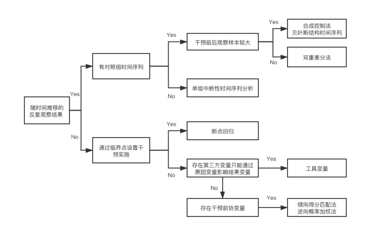
In some scenarios where random experiments cannot be carried out, synthetic control is required

When evaluating the effect of most operations and products, the most commonly used method is effect = post launch effect - pre launch effect. The biggest problem of this method lies in its key assumption that the online function or activity is the only variable that affects the effect. But just think about how unreasonable this assumption is.

The upgraded evaluation scheme may find a city or market to compare with the online cities. This idea is very similar to DID, but it also implies a key assumption, that is, cities with highly synchronous long-term change trends can be found, which is very difficult for businesses with strong regional characteristics.

A more upgraded version of the scheme may not need to find a city with a very similar change trend, and through a method similar to integrated learning, take multiple cities as inputs, and combine their own long-term time series fluctuations to fit a virtual reality without online strategy. It makes the search for highly synchronous cities change from a strong hypothesis to a weak hypothesis. Causal Impact is a concrete practice of this idea.

Causal Impact is based on Bayesian structure time series model. It will synthesize a variety of information inputs and combine its own time series to construct a virtual value whose strategy is not online, which is illustrated by a case.

1.2 Bayesian structure time series model

1.3 Google's Causal Impact

Data analysis (12): how to quantitatively evaluate the effect of marketing and product revision on business if AB test cannot be done

When the AB test cannot be performed, the indicators before and after the product is launched are generally directly selected for comparison after the product is launched. However, the indicators in different periods are affected differently, such as holidays and seasonal effects, which makes the selection of indicators before and after the launch more subjective.

In order to accurately quantify the effect of product revision, Google launched the open source project causalimpact toolkit. Based on the principle of synthetic control method, this method uses multiple control group data to build a Bayesian structure time series model, and constructs a comprehensive time series baseline after adjusting the size difference between the control group and the experimental group, so as to finally predict the counterfactual results. That is, if the product revision is not launched this time, how should the product indicators go. Then the impact of the product revision on the indicators is the difference between the real value (the indicator value after the product Revision) and the predicted value (the indicator value in the period when the product revision is not predicted).

In this method, you need to prepare:

1. Time series data

The daily, weekly or hourly value of the index to be evaluated is used as the input value of the method. The method will fit the index data before the product goes online to predict and obtain a new time series. Then the difference between the new time series and the real value of the index after the product goes online is the effect of the revision of the product.

2. Control group time series

Before prediction, the time series data with similar trend can be found and added to the model. It is known that the similar time series can be used as the trend effect in the prediction series, and the Pearson correlation coefficient can be used as the measure of time series similarity.

3. Data exploration required to achieve accurate prediction

The time series itself is composed of long-term trend, seasonal factors, periodic factors and random variation factors (as shown in the figure below). In order to predict accurately, it is necessary to identify these characteristics of historical data in order to predict the time series more accurately.

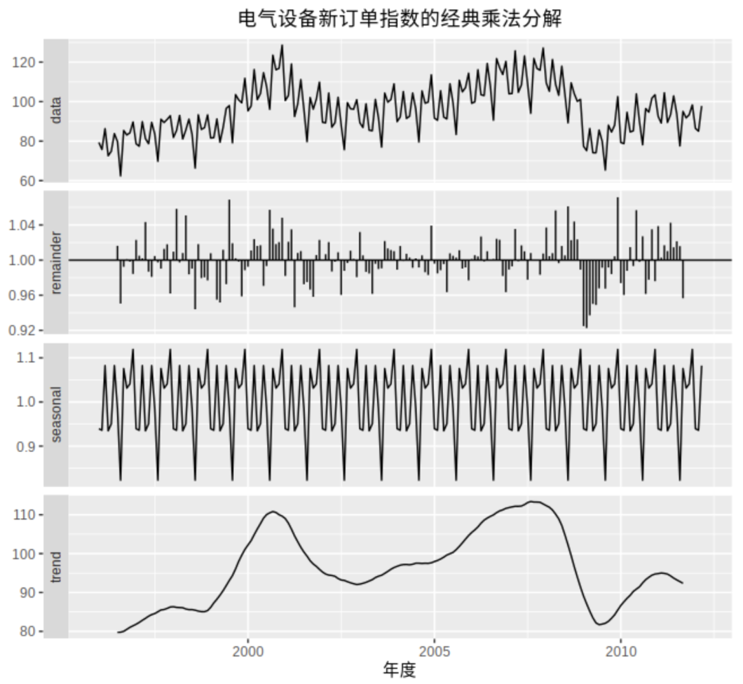
• Trend, that is, monotonicity in a certain period of time, generally speaking, the slope is fixed.
• Periodicity is very similar to seasonality, but its fluctuation time frequency is not fixed. Because its fluctuation frequency is not fixed, it is generally analyzed together with the trend without splitting. For example, the trend curve in the figure above falls to the bottom and then rebounds. This reciprocating motion is called periodicity.
• Seasonal, fixed length changes, just like the temperature changes in spring, summer, autumn and winter. For example, in the figure above, there will be a cycle every 12 months, and the values of each month in different years are roughly the same.
• During holidays, business is usually affected by holidays, which is finally reflected in the fluctuation of indicators. In order to identify the effect of holidays in the historical data, the simulation data should preferably have one year's historical data

2 some cases

2.1 timing selection of causalimpact

Non randomized effect evaluation method (2)

The takeout company launched strategy S in city A to improve the order matching rate. Since the strategy control experiment can not discriminate against riders, it cannot carry out AB experiment. It must be launched in full, and the strategy effect needs to be evaluated.

The construction of CausalImpact is divided into two steps:

·Controlled time series selection:

The dtw algorithm is used to select the time series most similar to the shopping list rate of city A. through the calculation of distance, the time series of shopping list rate before the intervention of city B is the closest to that of city A.

·By observing the fitting results, judge whether the strategy is consistent with the significant effect

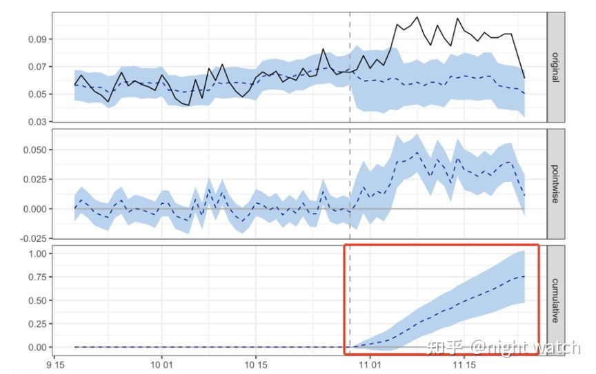
In the first figure (original), the black solid line is the actual results of city A before and after the strategy is launched, the blue dotted line is the results of city A fitted according to city B, that is, the results of city A when the simulated strategy is not launched, and the blue area is the confidence interval. The blue dotted line in the second figure (pointwise) shows the difference of order matching rate before and after the strategy of city A. It can be seen that after the strategy is launched, the difference of order matching rate is significantly positive. The blue dotted line in the third figure shows the cumulative value after the strategy is launched, which continues to increase. It can be seen that the strategy has an obvious positive effect.

The following figure shows the specific strategy effect:

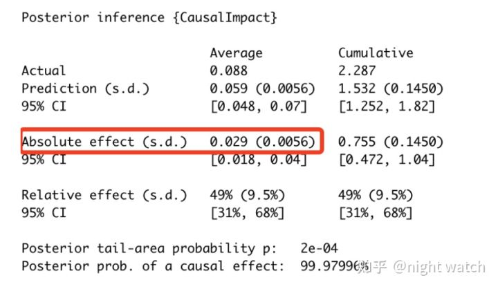
The average daily order splicing rate increased by 3pp

The author interprets more of the following figures:

• The first data module: the final average prediction value of the experiment is 0.059 and the average actual value is 0.088; while the cumulative prediction value is 1.532 and the cumulative actual value is 2.287; the average data range here is the time period after the above dotted line
• The second data module: after MCMC estimation, the absolute effect of the index increased by an average of 0.029 and a cumulative increase of 0.755; the relative effect increased by an average of 49% and a cumulative increase of 49%

CausalImpact has three main points:

• First, in the process of model fitting (original), the confidence interval of AA difference should always contain 0, which is equivalent to that the fitting error of the model is within our acceptable range. On the contrary, it indicates that the fitting error of the model is too large and the model is not credible;
• Second, after the strategy goes online (pointwise), whether the daily income level contains 0. If it contains 0, it means that the income is not significant;
• Third, the long-term benefits of strategies. Some strategies have novel effects and can not get long-term benefits, so we need to pay attention to the cumulative benefits for decision-making.

2.2 Japanese case: CausalImpact

CausalImpact

Thesis: https://ai.google/research/pubs/pub41854 python installation: https://github.com/dafiti/causalimpact Case address: https://github.com/rmizuta3/causalimpact/blob/master/causalimpact_restaurant.ipynb

Several traditional workflows for observation data (differential method + synthetic control method):

• Select more than one eligible control group
• Use the synthetic control method to select the control group (if there are more than one) The synthetic control method is a method to create a disposal group when it is supposed not to be disposed by making the weighted sum of multiple control groups as close as possible to the disposal group.
• Using DID, the treatment group was compared with the control group made in 2

Problems in the above workflow:

• Time series data generally produce autoregressive components, but DID assumes that each time point is independent and identically distributed.
• Since DID can only observe the difference between two points, for example, if the activity lasts for one week, the impact before the beginning and end of the activity cannot be observed separately.
• Due to the calculation of the two stages of synthetic control method → difference difference method, it is difficult to judge which stage has a greater impact on the error.

Introduction to CausalImpact method:

• Using the state space model, the control group without measures is generated from the control group, and the predicted value is calculated.
• Compare it with the value of the actual disposal group to calculate the causal effect.

Highlights of CausalImpact:

• Using the state space model, time series factors such as autoregressive components and seasonality can be considered
• The impact of each point in the time series can be confirmed
• The part of the synthetic control method and what DID are covered by a state space model, so it is easy to know which part has an error. Understand the uncertainty of the model.

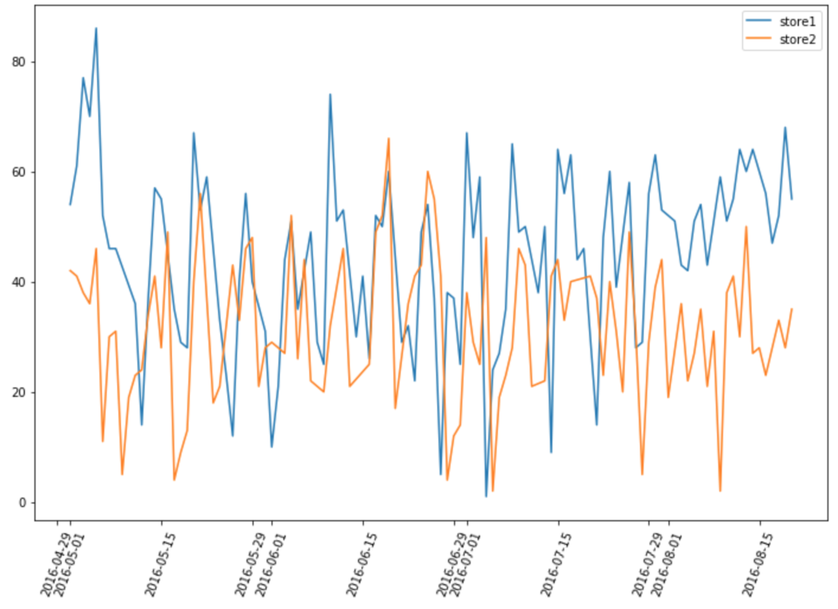
The data used is the same as the last time when the difference method was used. The number of visitors of Recruit Restaurant Visitor Forecasting restaurant was used to determine the impact effect of a store during the Yulan basin Festival (8 / 11-20).

The layout of the two stores is like this.

Here is the data processing process:

df=pd.read_csv("air_visit_data.csv",parse_dates=["visit_date"])

#Yuan, yuan, yuan, yuan, yuan, yuan, yuan, yuan, yuan, yuan, yuan, yuan, yuan, yuan, yuan, yuan, yuan, yuan, yuan, yuan, yuan, yuan, yuan, yuan, yuan, yuan, yuan, yuan, yuan, yuan, yuan, yuan, yuan, yuan, yuan, yuan, yuan, yuan, yuan, yuan, yuan, yuan, yuan, yuan, yuan, yuan, yuan, yuan, yuan, yuan, yuan, yuan, yuan, yuan, yuan, yuan, yuan, yuan, yuan, yuan, yuan, yuan, yuan, yuan, yuan
basedate=pd.DataFrame(list(pd.date_range('2016-05-01', '2016-08-20')))
basedate.columns=["visit_date"]

#Store designation and time limit
store1=df[df["air_store_id"]=="air_e55abd740f93ecc4"]
store1=store1[(store1["visit_date"]>="2016-05") & (store1["visit_date"]<="2016-08-20")]
store2=df[df["air_store_id"]=="air_1653a6c513865af3"]
store2=store2[(store2["visit_date"]>="2016-05") & (store2["visit_date"]<="2016-08-20")]

#Combination
store1.rename(columns={"visitors":"visitors_store1"},inplace=True)
store2.rename(columns={"visitors":"visitors_store2"},inplace=True)
data=pd.merge(basedate,store1[["visit_date","visitors_store1"]],on="visit_date",how="left")
data=pd.merge(data,store2[["visit_date","visitors_store2"]],on="visit_date",how="left")
data=data.interpolate() #Under damaged linear repair
data=data.set_index("visit_date")

pre_period and post_period represents observation period and prediction period respectively; Because of the impact in terms of weeks, nseason here is 7.

from causalimpact import CausalImpact
pre_period = ['2016-05-01', '2016-08-10']
post_period = ['2016-08-11', '2016-08-20']
ci = CausalImpact(data, pre_period, post_period,nseasons=[{'period': 7}],trend=True)
print(ci.summary())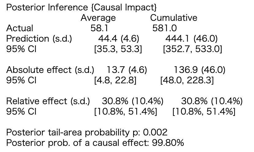

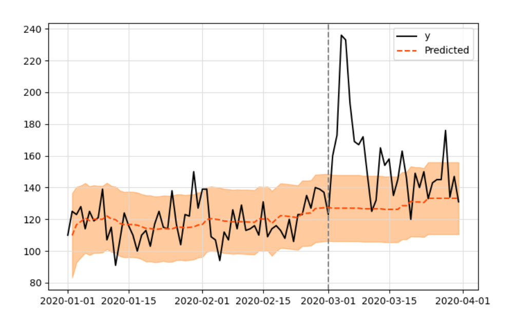
The effect of Yulan basin festival was 13.7 people on average, and 137 people accumulated in 10 days. When using DID, the value is 13.5 people, so the value is almost the same. The 95% confidence interval is also calculated. From a cumulative view of 48.0 ~ 228.3, it can be seen that the structural model is not stable. It's good to see how uncertain the results are.

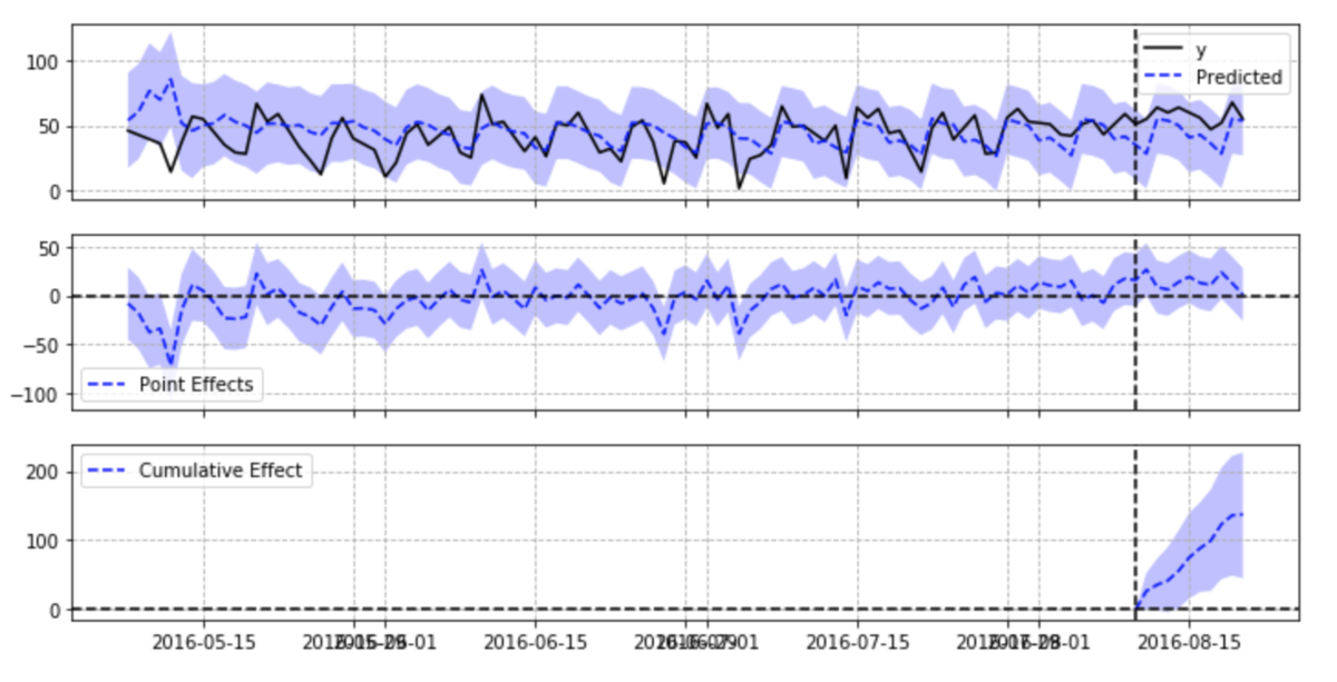
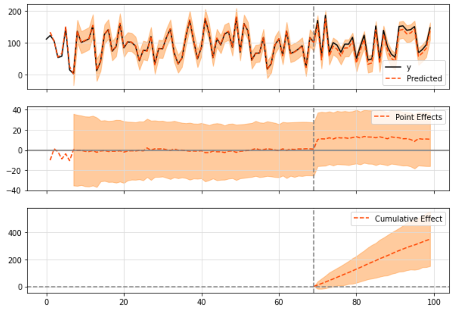
In the first figure, y is the disposal group, Predicted is the Predicted value of the state space model, and the colored part is the confidence interval of the Predicted value. The second chart represents the y-Predicted of the first chart. The third chart shows the cumulative sum of y-Predicted during disposal.

By the way, CausalImpact includes UnobservedComponents, which can view the results of the state space model itself.

ci.trained_model.summary()

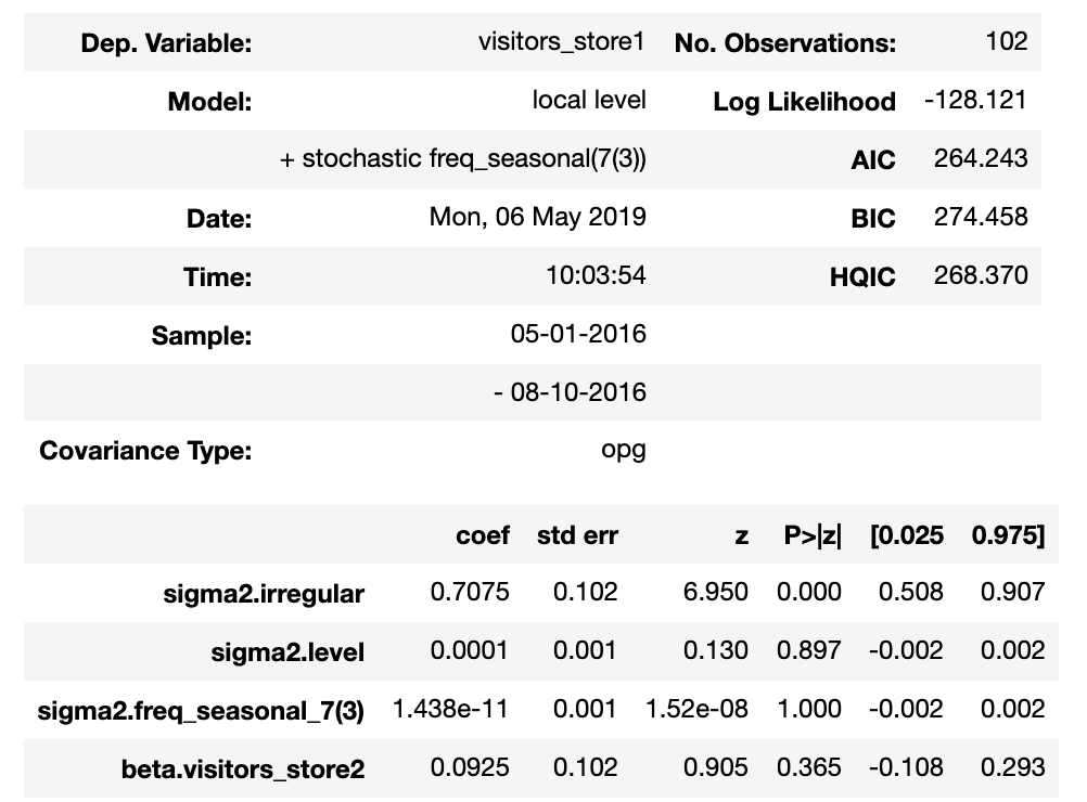
Because the observation error of the created state space model is very large, the confidence interval becomes very wide.

CausalImpact usually needs to enter the control group, but it can also be used if not. In this case, the state space model is created by fitting from the time sequence of the experimental group.

pre_period = ['2016-05-01', '2016-08-10']
post_period = ['2016-08-11', '2016-08-20']
ci = CausalImpact(data.iloc[:,0], pre_period, post_period,nseasons=[{'period': 7}])
ci.plot(figsize=(12, 6))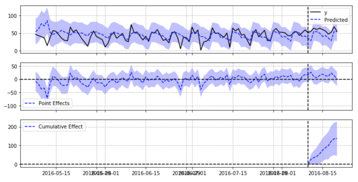

This example is not much different from the results of adding the control group. If the control group can input multiple data, the results may be more stable.

I'm glad to get the confidence interval of the effect Because each point can be speculated, the changes in the processing interval can also be seen, which seems good. It may not work when you cannot enter multiple objects.

2.3 [translation] R language case: an R package for causal information using Bayesian structural time series models

An R package for causal inference using Bayesian structural time-series models

The package is designed to make counterfactual reasoning as simple as fitting regression model, but it is much more powerful when the above assumptions are met. The package has only one entry point, the function CausalImpact(). Given a response time series and a set of control time series, the function constructs a time series model, performs a posteriori reasoning on the counterfactual, and returns a CausalImpact object. The results can be summarized in tables, text descriptions or charts.

# Create data
set.seed(1)
x1 <- 100 + arima.sim(model = list(ar = 0.999), n = 100)
y <- 1.2 * x1 + rnorm(100)
y[71:100] <- y[71:100] + 10
data <- cbind(y, x1)


pre.period <- c(1, 70)
post.period <- c(71, 100)
# Drawing
impact <- CausalImpact(data, pre.period, post.period)
plot(impact)

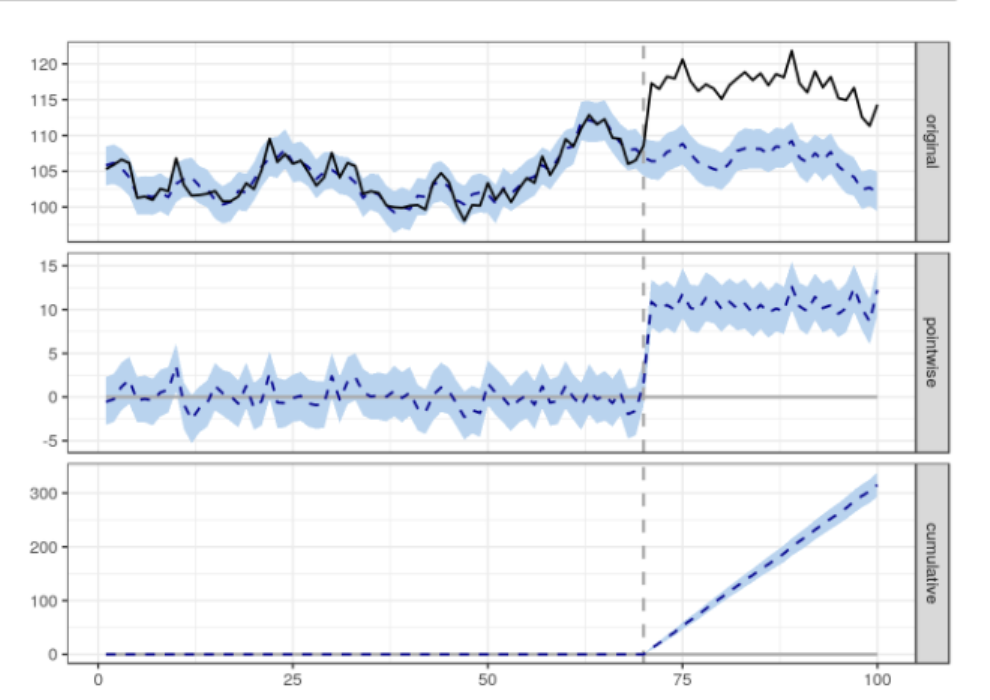
By default, the drawing contains three panels. The first panel shows the data and a counterfactual prediction of the post-treatment period. The second panel shows the difference between the observed data and the counterfactual prediction. This is the pointwise causal effect estimated by the model. The third group added the point by point contributions of the second group to obtain the cumulative effect of the intervention.

Remember, again, all the above inferences depend on the assumption that the covariates themselves are not affected by the intervention. The model also assumes that the relationship between the covariates established in the previous period and the processing time series remains stable throughout the latter period.

3 Official: TensorFlow Causal Impact

Official website address: getting_started

3.1 background

The working principle of the impact model developed by Google is to fit the Bayesian structure time series model with the observed data. These data are later used to predict what results will be produced if there is no intervention in a given time period, as shown in the figure below:

The idea is to use the prediction of the fitted model (expressed in orange) as a reference to what may be observed without intervention.

Bayesian structure time series model can be expressed by the following formula:

y_t = Z^T_t\alpha_t + \beta X_t + G_t\epsilon_t a_{t+1} = T_t\alpha_t + R_t\eta_t

\epsilon_t \sim \mathcal{N}(0, \sigma_t^2)

\eta_t \sim \mathcal{N}(0, Q_t)

a, also known as the "state" of the series, yt is the linear combination of states plus the linear regression of covariate X (and the measurement noise following the zero mean normal distribution) ϵ).

By changing matrices Z, T, G and R, we can model several different behaviors for time series (including the more famous ARMA or ARIMA).

In this package (as in Google's R package), you can choose any time series model you want to fit your data (described in detail below). If the model is not used as input, a local level is built by default, which means that yt is expressed as:

y_t = \mu_t + \gamma_t + \beta X_t + \epsilon_t

\mu_{t+1} = \mu_t + \eta_{\mu, t}

• \mu_t variable, autoregressive process, any given time point is first determined by the random walk component \ mu_t # modeling, also known as "local level" component, does not add any additional covariates in the autoregressive link
• Gamma for simulating seasonal components_ T variable
• We have weight \ beta X_t this is a linear regression of covariates, which is further helpful to explain the observed data. The more significant this component is in the prediction task, \ Mu_ The smaller the influence of T variable is, there is a relative relationship.
• Parameters \ epsilon_t) simulation and measurement y_t correlated noise, which follows zero mean and \ sigma_ Normal distribution of {\ epsilon} standard deviation.

Generate data:

%matplotlib inline

import sys
import os


sys.path.append(os.path.abspath('../'))


import numpy as np
import pandas as pd
import tensorflow as tf
import tensorflow_probability as tfp
import matplotlib.pyplot as plt
from causalimpact import CausalImpact


tfd = tfp.distributions
plt.rcParams['figure.figsize'] = [15, 10]

# Generate data
# This is an example presented in Google's R code.
# Uses TensorFlow Probability to simulate a random walk process.
observed_stddev, observed_initial = (tf.convert_to_tensor(value=1, dtype=tf.float32),
                                     tf.convert_to_tensor(value=0., dtype=tf.float32))
level_scale_prior = tfd.LogNormal(loc=tf.math.log(0.05 * observed_stddev), scale=1, name='level_scale_prior')
initial_state_prior = tfd.MultivariateNormalDiag(loc=observed_initial[..., tf.newaxis], scale_diag=(tf.abs(observed_initial) + observed_stddev)[..., tf.newaxis], name='initial_level_prior')
ll_ssm = tfp.sts.LocalLevelStateSpaceModel(100, initial_state_prior=initial_state_prior, level_scale=level_scale_prior.sample())
ll_ssm_sample = np.squeeze(ll_ssm.sample().numpy())

x0 = 100 * np.random.rand(100)
x1 = 90 * np.random.rand(100)
y = 1.2 * x0 + 0.9 * x1 + ll_ssm_sample
y[70:] += 10
data = pd.DataFrame({'x0': x0, 'x1': x1, 'y': y}, columns=['y', 'x0', 'x1'])

data.plot()
plt.axvline(69, linestyle='--', color='k')
plt.legend();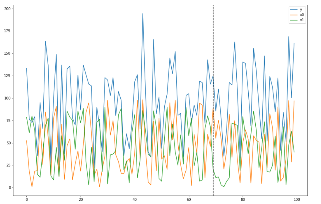

3.2 default model

Use default model:

pre_period = [0, 69]
post_period = [70, 99]
ci = CausalImpact(data, pre_period, post_period)

ci.plot()

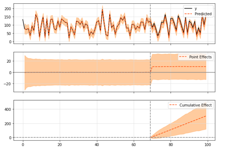
When drawing results, three kinds of graphics are printed by default:

• "Original" series and expected series
• "Point effect" (i.e. the difference between the original sequence and the predicted sequence)
• Finally, the "cumulative" effect, which is basically the sum of point effects accumulated over time.

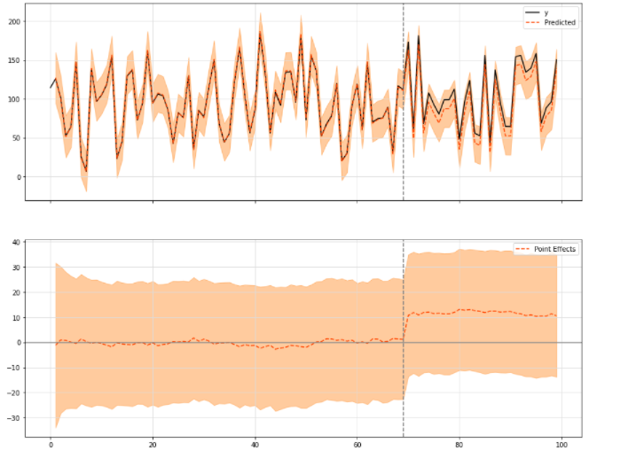
You can choose to print some of the three modules in the above figure:

ci.plot(panels=['original', 'pointwise'], figsize=(15, 12))

In order to see the general results and figures, you can call the summary method with default input or "report", which will print out a more detailed explanation of the observed effects:

print(ci.summary())

The result is:

Posterior Inference {Causal Impact}
                          Average            Cumulative
Actual                    106.01             3180.15
Prediction (s.d.)         96.16 (3.6)        2884.67 (107.86)
95% CI                    [89.16, 103.25]    [2674.67, 3097.47]

Absolute effect (s.d.)    9.85 (3.6)         295.49 (107.86)
95% CI                    [2.76, 16.85]      [82.69, 505.48]

Relative effect (s.d.)    10.24% (3.74%)     10.24% (3.74%)
95% CI                    [2.87%, 17.52%]    [2.87%, 17.52%]

Posterior tail-area probability p: 0.0
Posterior prob. of a causal effect: 99.6%

For more details run the command: print(impact.summary('report'))

For example, we can see here that the absolute effect observed is about 9, and its prediction varies from 2 to 15 with a 95% confidence interval.

The difference in this confidence interval is still quite large

When observing these results, a very important number is the p value, The probability of causal effect (not just noise) can be proved by P value. So, as a hypothesis test.

If you want a more detailed summary, run the following command:

print(ci.summary(output='report'))

See the following for details:

Analysis report {CausalImpact}


During the post-intervention period, the response variable had
an average value of approx. 106.01. By contrast, in the absence of an
intervention, we would have expected an average response of 96.16.
The 95% interval of this counterfactual prediction is [89.16, 103.25].
Subtracting this prediction from the observed response yields
an estimate of the causal effect the intervention had on the
response variable. This effect is 9.85 with a 95% interval of
[2.76, 16.85]. For a discussion of the significance of this effect,
see below.

ci also has a lot of information. For example, for each sequence:

ci.inferences.head()

print('Mean value of noise observation std: ', ci.model_samples[0].numpy().mean())
print('Mean value of level std: ', ci.model_samples[1].numpy().mean())
print('Mean value of linear regression x0, x1: ', ci.model_samples[2].numpy().mean(axis=0))

3.3 set some specifications

3.3. 1 set a priori standard deviation

Some numerical specifications can also be set here, such as controlling the a priori standard deviation within a certain range. Here is an example:

ci = CausalImpact(data, pre_period, post_period, model_args={'prior_level_sd':0.1})
ci.plot(figsize=(15, 12))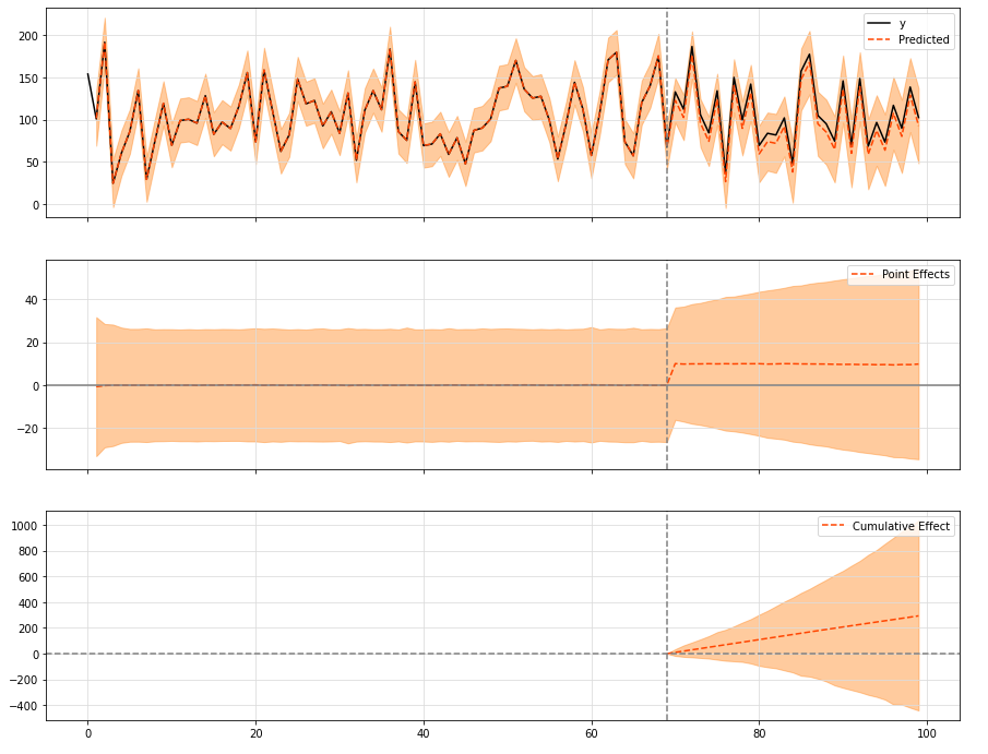

The default value is 0.01, which means that the data performs well, the variance is small, and the covariates can be well explained. If it turns out that this is not the case for a given input data, the a priori value of the local standard deviation can be changed to reflect this pattern in the data. For the value of 0.1, we basically mean that there is a stronger random walk component in the data, which cannot be explained by the covariate itself.

3.3. 2 set seasonal factors

observed_stddev, observed_initial = (5., 0.)
num_seasons = 7

drift_scale_prior = tfd.LogNormal(loc=tf.math.log(.01 * observed_stddev), scale=1.)
initial_effect_prior = tfd.Normal(loc=observed_initial, scale=tf.abs(observed_initial) + observed_stddev)
initial_state_prior = tfd.MultivariateNormalDiag(loc=tf.stack([initial_effect_prior.mean()] * num_seasons, axis=-1),
                                                 scale_diag=tf.stack([initial_effect_prior.stddev()] * num_seasons, axis=-1))

s_ssm = tfp.sts.SeasonalStataeSpaceModel(
    num_timesteps=100,
    num_seasons=num_seasons,
    num_steps_per_season=1,
    drift_scale=drift_scale_prior.sample(),
    initial_state_prior=initial_state_prior
)

plt.plot(s_ssm.sample());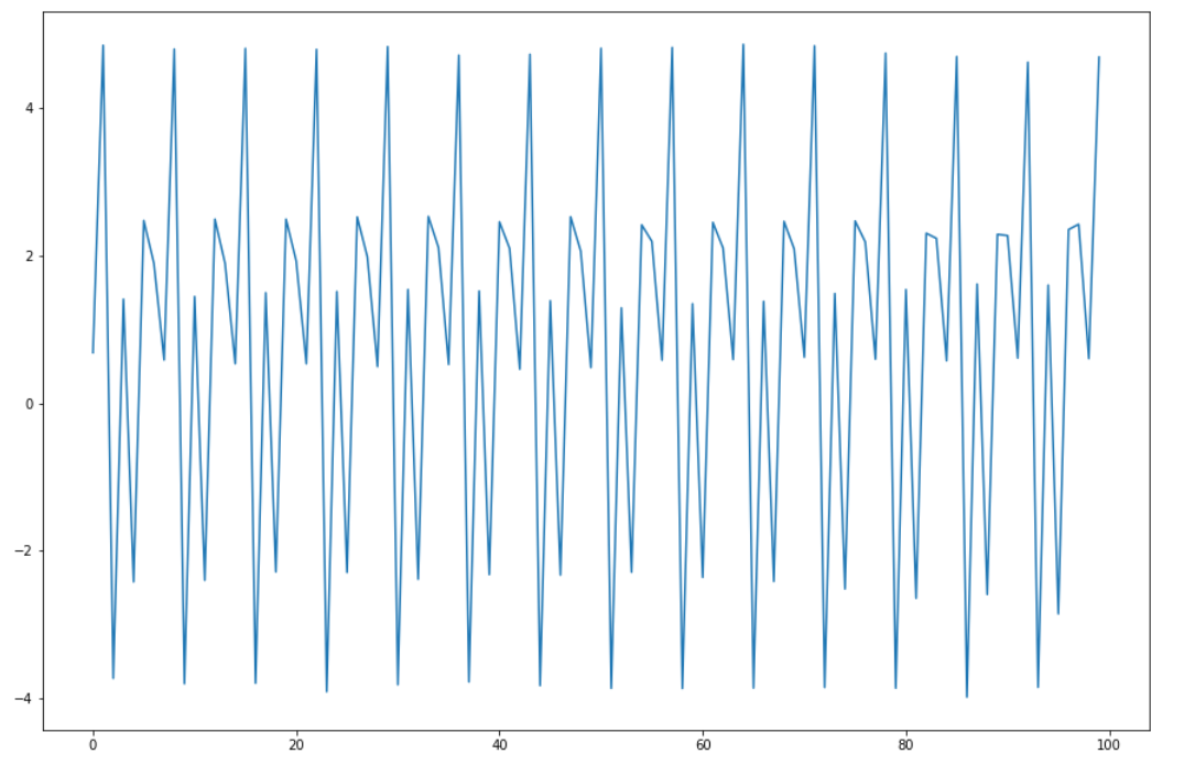

season_data = data.copy()
season_data['y'] += np.squeeze(s_ssm.sample().numpy())

ci = CausalImpact(season_data, pre_period, post_period, model_args={'nseasons': 7})

print(ci.summary())

ci.plot()

Output:

Posterior Inference {Causal Impact}
                          Average            Cumulative
Actual                    103.22             3096.61
Prediction (s.d.)         91.52 (3.48)       2745.52 (104.37)
95% CI                    [84.63, 98.26]     [2538.75, 2947.89]

Absolute effect (s.d.)    11.7 (3.48)        351.09 (104.37)
95% CI                    [4.96, 18.6]       [148.72, 557.85]

Relative effect (s.d.)    12.79% (3.8%)      12.79% (3.8%)
95% CI                    [5.42%, 20.32%]    [5.42%, 20.32%]

Posterior tail-area probability p: 0.0
Posterior prob. of a causal effect: 99.9%

For more details run the command: print(impact.summary('report'))

and