be careful:
- When you study this series of tutorials again, you should have installed ROS and need to have some basic knowledge of ROS
ubuntu version: 20.04
ros version: noetic
Course review
Developing course of Kitti with ROS1 combined with autopilot data set (I) Kitti data introduction and visualization
ROS1 releases pictures in combination with Kitti development tutorial (II) of automatic driving data set
ROS1 releases point cloud data in combination with Kitti development tutorial (III) of automatic driving data set
ROS1 combines Kitti development tutorial (IV) of automatic driving data set to draw its own car model and camera field of view
ROS1 releases IMU data in combination with Kitti development tutorial (V) of autopilot data set
ROS1 releases GPS data in combination with Kitti development tutorial (VI) of autopilot data set
ROS1 combined with Kitti development tutorial of automatic driving data set (VII) Download Image Annotation materials and read the display
ROS1 draws a 2D detection box in combination with Kitti development tutorial (8) of automatic driving data set
1. Preliminary preparations
Open the Jupyter Notebook, enter the source code address, and create a new source code file named plot3d ipynb
Lidar data visualization open source website
Basic knowledge of rotation matrix
2. Draw the 3D detection frame of one of the objects
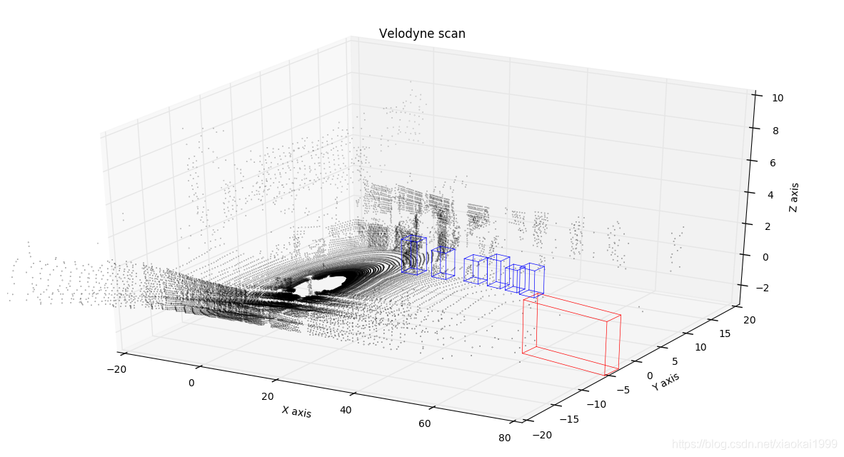
So far, pioneers have opened the project Visualizing lidar data , the display effect is very good. Through the author's tutorial, the effect shown in the figure below can also be realized.
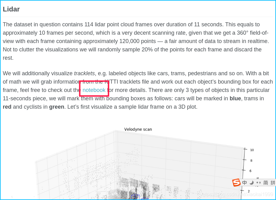
First, find the link as shown in the figure below on the project page. You can see that the original author has provided some key codes. We can realize the 3D detection box display in the first step by changing its source code (the following program can synthesize a whole function from beginning to end and directly put it into the Jupiter notebook):
2.1 loading point cloud data function
This procedure is the same as the previous procedure, so I won't repeat it.
import numpy as np
import os
BASE_PATH = "/home/mckros/kitti/RawData/2011_09_26/2011_09_26_drive_0005_sync/"
def read_point_cloud():
    point_cloud = np.fromfile(os.path.join(BASE_PATH, "velodyne_points/data/%010d.bin"%0), dtype=np.float32).reshape(-1,4)
    return point_cloud
2.2 point cloud rendering function
The following program provides a point cloud drawing function, which is slightly different from the original author's program. Here, some changes have been made according to the author's needs.
The main usage parameters of the function are described as follows:
ax: matplotlib Sketchpad
points: read_ point_ Point cloud data read by cloud()
Title: Sketchpad title
Axes: [0,1,2] represent xyz three axes respectively
point_size: point cloud size
xlim3d: the X axis limits the range of angles in 3D display
ylim3d: the Y axis limits the range of angles under 3D display
zlim3d: the Z axis limits the range of angles in 3D display
import matplotlib.pyplot as plt
from mpl_toolkits.mplot3d import Axes3D

def draw_point_cloud(ax, points, title, axes=[0, 1, 2], point_size=0.2, xlim3d=None, ylim3d=None, zlim3d=None):
    """
    Convenient method for drawing various point cloud projections as a part of frame statistics.
    """
    # Sets xyz the point cloud range for the three axes
    axes_limits = [
        [-20, 80], # X axis range
        [-20, 20], # Y axis range
        [-3, 5]    # Z axis range
    ]
    axes_str = ['X', 'Y', 'Z']
    # Suppress the display of the grid behind
    ax.grid(False)
    # Create scatter chart [1]:xyz dataset, [2]: size of point cloud, [3]: reflectance data of point cloud, [4]: grayscale display
    ax.scatter(*np.transpose(points[:, axes]), s=point_size, c=points[:, 3], cmap='gray')
    # Set the title of the sketchpad
    ax.set_title(title)
    # Set x-axis title
    ax.set_xlabel('{} axis'.format(axes_str[axes[0]]))
    # Set y-axis title
    ax.set_ylabel('{} axis'.format(axes_str[axes[1]]))
    if len(axes) > 2:
        # Set limit angle
        ax.set_xlim3d(*axes_limits[axes[0]])
        ax.set_ylim3d(*axes_limits[axes[1]])
        ax.set_zlim3d(*axes_limits[axes[2]])
        # Set the background color to RGBA format, and the current parameters are displayed transparently
        ax.xaxis.set_pane_color((1.0, 1.0, 1.0, 0.0))
        ax.yaxis.set_pane_color((1.0, 1.0, 1.0, 0.0))
        ax.zaxis.set_pane_color((1.0, 1.0, 1.0, 0.0))
        # Set z-axis title
        ax.set_zlabel('{} axis'.format(axes_str[axes[2]]))
    else:
        # 2D limit angle, only xy axis
        ax.set_xlim(*axes_limits[axes[0]])
        ax.set_ylim(*axes_limits[axes[1]])
    # User specified limits
    if xlim3d!=None:
        ax.set_xlim3d(xlim3d)
    if ylim3d!=None:
        ax.set_ylim3d(ylim3d)
    if zlim3d!=None:
        ax.set_zlim3d(zlim3d)
2.3 display point cloud
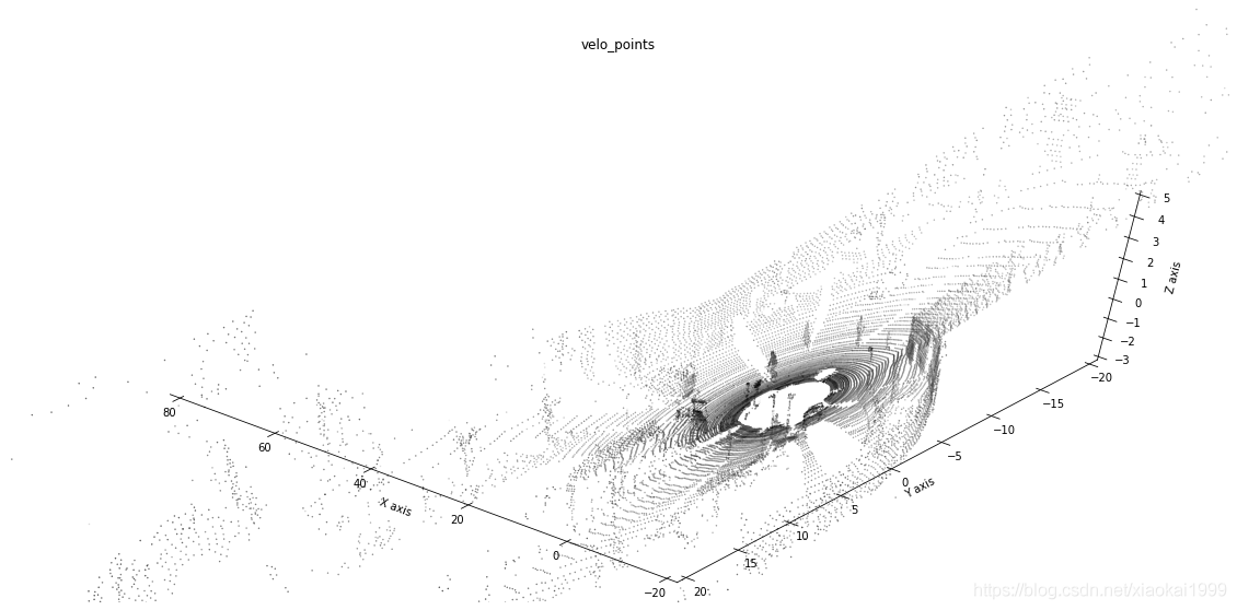
Enter the following program in the Jupiter notebook to display the most basic 3D point cloud. If you want to get a good-looking point cloud display, you need to optimize it by adjusting your own parameters..
# Get point cloud data in dataset
point_cloud = read_point_cloud()
# Draw 3D point cloud data and create a graphic Sketchpad with a size of 20 * 10
fig = plt.figure(figsize=(20, 10))
# Add the first sub image of 1 * 1 grid to the drawing board, which is a 3D image
ax = fig.add_subplot(111, projection='3d')
# Change the viewing angle of the drawn image, that is, the position of the camera. elev is the Z-axis angle and azim is the (x,y) angle
ax.view_init(60,130)
# Draw a point cloud on the drawing board to display the data, point_ The larger the cloud [:: x] x value, the more sparse the points displayed
draw_point_cloud(ax, point_cloud[::5], "velo_points")
The effect is as follows:
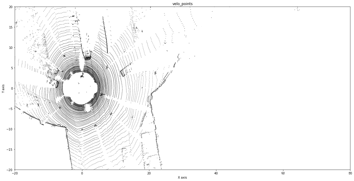
It is also very simple to obtain 2D point cloud. The code is as follows:
# The same is to create a canvas, but this function is in place in one step
fig, ax = plt.subplots(figsize=(20,10))
# Draw the point cloud in the direction of 2D [x,y] axis
draw_point_cloud(ax, point_cloud[::5], "velo_points", axes=[0, 1])
The effect is as follows:
2.4 obtaining label data
We need to get the label_02 data, where bbox_left,bbox_top,bbox_right,bbox_ The four parameters of bottom are the four vertices of the 2D detection box mentioned in the previous tutorial. This time, we will use dimensions_height,dimensions_width,dimensions_length,location_x,location_y,location_z,rotation_y these 7 parameters are used to calculate the 8 vertex coordinates of the 3D detection frame.
Because these codes have been analyzed before, I won't repeat them today.
import pandas as pd
LABEL_NAME = ["frame", "track id", "type", "truncated", "occluded", "alpha", "bbox_left", "bbox_top", "bbox_right", "bbox_bottom", "dimensions_height", "dimensions_width", "dimensions_length", "location_x", "location_y", "location_z", "rotation_y"]
df = pd.read_csv(os.path.join(BASE_PATH, "label_02/0000.txt"), header=None, sep=" ")
df.columns = LABEL_NAME
df.loc[df.type.isin(['Van','Car','Truck']),'type'] = 'Car'
df = df[df.type.isin(['Car','Cyclist','Pedestrian'])]
df
The output results are as follows:

2.5 calculate 8 vertex coordinates of 3D detection frame
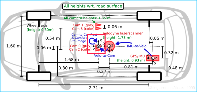
In the Kitti dataset, dimensions_height,dimensions_width,dimensions_length,location_x,location_y,location_z,rotation_y these seven parameters are marked with Cam2 as the datum coordinate system. Through the following analysis, 3DBox in Cam2 can be calculated first.
-
Firstly, according to the equipment installation drawing provided by Kitti, the coordinate system of Cam2 can be seen as follows:
-
Therefore, we can roughly draw the most ideal model and preliminarily calculate the vertex coordinates, that is, yaw=0, as shown below.
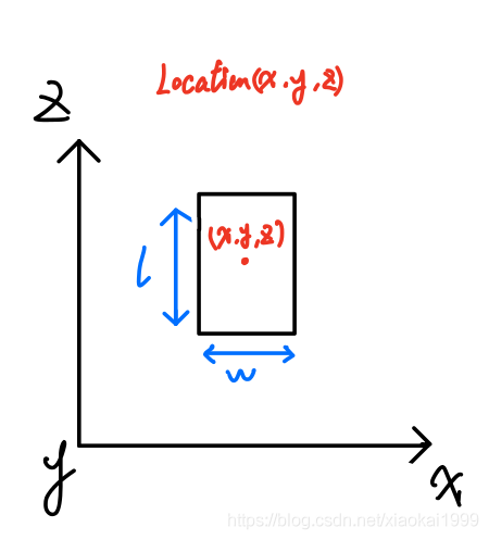
You can see the God perspective model of the object drawn according to the coordinate system of Cam2, because you know the dimensions_height,dimensions_width,dimensions_length, so it is easy to draw the length and width of the object_ x,location_y,location_z represents the coordinates of the center point of the object model, and then we can easily get the coordinates of 8 vertices, as shown in the following formula:
( x ± w 2 , y , z ± l 2 ) (x\pm \frac{w}{2},y,z\pm \frac{l}{2}) (x±2w,y,z±2l)
You can replace it with the difference relative to the Location coordinate system, as follows:
x
c
o
r
n
e
r
s
=
(
l
2
,
l
2
,
−
l
2
,
−
l
2
,
l
2
,
l
2
,
−
l
2
,
−
l
2
)
xcorners = (\frac{l}{2},\frac{l}{2},-\frac{l}{2},-\frac{l}{2},\frac{l}{2},\frac{l}{2},-\frac{l}{2},-\frac{l}{2})
xcorners=(2l,2l,−2l,−2l,2l,2l,−2l,−2l)
y c o r n e r s = ( 0 , 0 , 0 , 0 , − h , − h , − h , − h ) ycorners = (0,0,0,0,-h,-h,-h,-h) ycorners=(0,0,0,0,−h,−h,−h,−h)
z
c
o
r
n
e
r
s
=
(
w
2
,
−
w
2
,
−
w
2
,
w
2
,
w
2
,
−
w
2
,
−
w
2
,
w
2
)
zcorners = (\frac{w}{2},-\frac{w}{2},-\frac{w}{2},\frac{w}{2},\frac{w}{2},-\frac{w}{2},-\frac{w}{2},\frac{w}{2})
zcorners=(2w,−2w,−2w,2w,2w,−2w,−2w,2w)
However, this is only the coordinate obtained when yaw=0. Generally, objects will not be placed normally, and there will be a rotation angle. Rotation is also provided in kitti dataset_ y is the rotation angle of the object around the y axis, similar to the following figure:
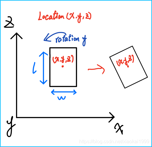
At this time, you need to convert the coordinates when yaw=0 to yaw by point multiplication through the rotation matrix= The coordinates at 0 rotate around the Y axis, so the rotation matrix is:
[
c
o
s
(
y
a
w
)
0
s
i
n
(
y
a
w
)
0
1
0
s
i
n
(
y
a
w
)
0
c
o
s
(
y
a
w
)
]
(2)
\left[ \begin{matrix} cos(yaw) & 0 & sin(yaw) \\ 0 & 1 & 0 \\ sin(yaw) & 0 & cos(yaw) \end{matrix} \right]\tag{2}
⎣⎡cos(yaw)0sin(yaw)010sin(yaw)0cos(yaw)⎦⎤(2)
The code is as follows:
def compute_3d_box_cam2(h, w, l, x, y, z, yaw):
    # Calculate rotation matrix
    R = np.array([[np.cos(yaw), 0, np.sin(yaw)], [0, 1, 0], [-np.sin(yaw), 0, np.cos(yaw)]])
    # xyz of 8 vertices
    x_corners = [l/2,l/2,-l/2,-l/2,l/2,l/2,-l/2,-l/2]
    y_corners = [0,0,0,0,-h,-h,-h,-h]
    z_corners = [w/2,-w/2,-w/2,w/2,w/2,-w/2,-w/2,w/2]
    # Rotation matrix dot multiplication (3,8) vertex matrix
    corners_3d_cam2 = np.dot(R, np.vstack([x_corners,y_corners,z_corners]))
    # Add the location center point to obtain the coordinates of 8 vertices after rotation
    corners_3d_cam2 += np.vstack([x,y,z])
    return corners_3d_cam2
# Calculate 3DBox in cam2
corners_3d_cam2 = compute_3d_box_cam2(*df.loc[2,['dimensions_height','dimensions_width','dimensions_length','location_x','location_y','location_z','rotation_y']])
2.6 draw the original appearance of the object
fig = plt.figure(figsize=(20,10))
ax = fig.add_subplot(111, projection='3d')
ax.view_init(40,150)
draw_box(ax,(corners_3d_cam2))
The effects are as follows:
2.7 transformation from CAM2 coordinate system to velo coordinate system
Download the calibration translator: kitti_util.py
The code is as follows:
from kitti_util import *
# Reading calibration conversion data
calib = Calibration("/home/mckros/kitti/RawData/2011_09_26/", from_video=True)
# Cam 2 to velo coordinate system
corners_3d_velo = calib.project_rect_to_velo(corners_3d_cam2.T).T
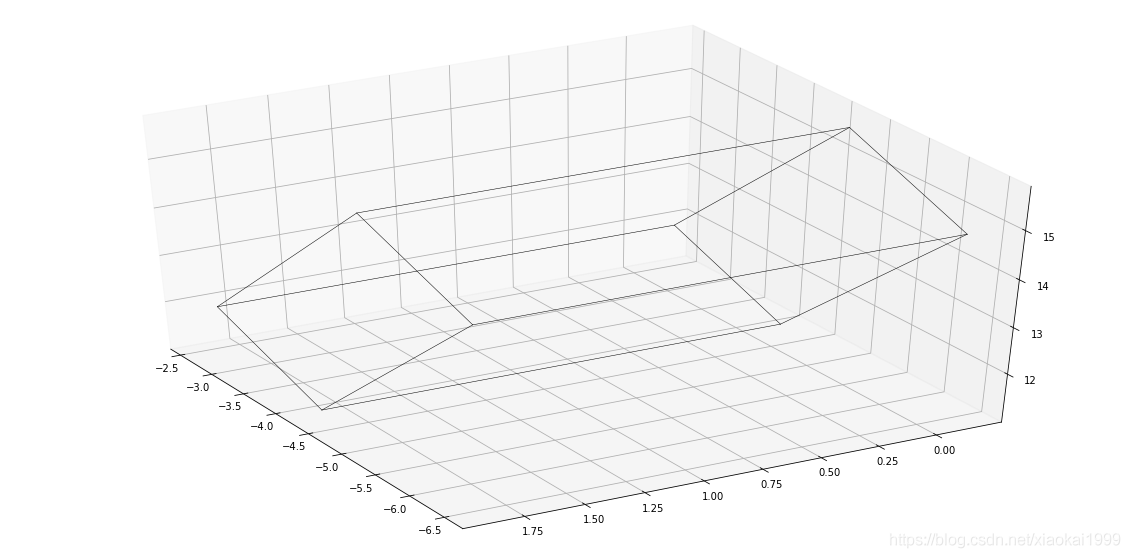
2.8 draw the converted object detection box
fig = plt.figure(figsize=(20,10))
ax = fig.add_subplot(111, projection = '3d')
ax.view_init(40,150)
draw_box(ax,corners_3d_velo)
The effect is as follows:

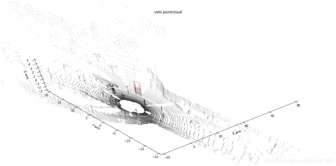
2.9 draw the detection box with the point cloud
# Combined with point cloud
fig = plt.figure(figsize=(20,10))
ax = fig.add_subplot(111, projection = '3d')
ax.view_init(70,230)
draw_point_cloud(ax,point_cloud[::5],"velo pointcloud")
draw_box(ax,corners_3d_velo,color='red')
The effect is as follows:
From God's perspective
fig, ax = plt.subplots(figsize=(20,10))
draw_point_cloud(ax,point_cloud[::5],"velo pointcloud",axes=[0,1])
draw_box(ax,corners_3d_velo,color='red',axes=[0,1])
The effect is as follows:

epilogue
This article is also based on the author's learning and use experience. It is highly subjective. If there is anything wrong or unclear, please leave a message in the comment area~
In order to further discuss problems with readers, a wechat group has been established to answer questions or discuss problems together.
Add group link
✌Bye