ElasticSearch node type
Master node: node master:true;
Data node: node data:true;
Client node
- When the configuration of the master node and the data node is false, the node is immature and mischievous, processing routing requests, processing searches, distributing index operations, etc; It shows the effect of load balancing;
- An independent client node is very useful in a large cluster. It coordinates the master node and the data section
The client node can join the cluster to get the status of the cluster, and the requests can be routed directly according to the status of the cluster.
Data node
When node When data is true, the data node is mainly the node that stores index data, mainly adding, deleting, modifying, querying, aggregating and so on. Data nodes have high requirements for CPU, memory and IO.
Master node
-
The primary node is responsible for the contents related to cluster operation; For example, create and delete indexes, track which nodes are part of the cluster, and determine which partitions are assigned to related nodes.
-
A stable master node is very important to the health of the cluster. By default, all nodes in a cluster may be selected as the master node. Indexing data, searching and querying operations will occupy a lot of cpu, memory and io resources. In order to ensure the stability of a cluster, it is necessary to separate
Master node and data node are a better choice. -
Usually, more than three nodes are set in the cluster as master nodes. These nodes are only responsible for becoming the master node and maintaining the state of the whole cluster. Then set up a batch of data nodes according to the data volume. These nodes are only responsible for storing data and provide indexing and query services in the later stage. In this way, if user requests are frequent, the pressure on these nodes will be relatively large. A batch of client nodes can be set up in the cluster to process user requests, realize request forwarding and load balancing;
The underlying principle of ES document score calculation
boolean model
Filter out the doc containing the specified term according to the user's query conditions;
 query "hello world" ‐‐> hello / world / hello & world
 bool ‐‐> must/must not/should ‐‐> filter ‐‐> contain / Not included / May contain
 doc ‐‐> No score ‐‐> Positive or negative true or false ‐‐> In order to reduce the subsequent calculation doc Quantity and improvement
relevance score algorithm
Calculate the association matching degree between the text in an index and the search text;
Elasticsearch uses the term frequency/inverse document frequency algorithm, referred to as
TF/IDF algorithm
Term frequency: how many times each term in the search text appears in the field text, and the more times it appears
More, the more relevant
 Search request: hello world
 doc1: hello you, and world is very good
  doc2: hello, how are you
Inverse document frequency: each term in the search text appears in all documents in the entire index
How many times, the more times, the less relevant
Search request: hello world
doc1: hello, study is very good
doc2: hi world, how are you
For example, there are 10000 documents in the index, and the word hello appears in all documents
1000 times; The word world appears 100 times in all document s
Field length norm: field length. The longer the field, the weaker the correlation
Search request: hello world
 doc1: { "title": "hello article", "content": "...... N Words" }
 doc2: { "title": "my article", "content": "...... N A word, hi world" }
hello world appears the same number of times in the whole index, doc1 is more relevant and title field is shorter
Analyze a document_ How is score calculated
GET /es_db/_doc/1/_explain
 {
 "query": {
 "match": {
 "remark": "java developer"
 }
 }
 }
Word splitter workflow
- Segmentation, normalization
Give you a sentence, and then split the sentence into single words one by one. At the same time, normalize each word (tense conversion, singular and plural conversion), word splitter recall, recall rate: when searching, increase the number of results that can be searched
character filter: Before word segmentation of a text, preprocess it first. For example, the most common is filtering html
 Label(<span>hello<span> ‐‐> hello),& ‐‐> and(I&you ‐‐> I and you)

tokenizer: Participle, hello you and me ‐‐> hello, you, and, me
A word splitter is very important. It processes a paragraph of text in various ways, and the final processed result will be used to create an inverted word
Row index
ES built in word splitter
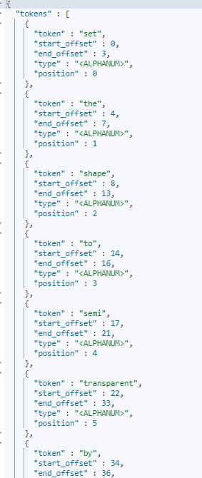
- standard analyzer: set, the, shape, to, semi, transparent, by, calling, set_trans, 5 (standard by default)
- simple analyzer: set, the, shape, to, semi, transparent, by, calling, set, trans
- whitespace analyzer: Set, the, shape, to, semi‐transparent, by, calling, set_trans(5)
- whitespace analyzer: Set, the, shape, to, semi‐transparent, by, calling, set_tr
ans(5)
//test
POST _analyze
{
  "analyzer": "standard",
  "text": "Set the shape to semi‐transparent by calling set_trans(5)"
}
Custom word splitter
- Default word breaker standard
standard tokenizer: Segmentation with word boundaries
standard token filter: Don't do anything?
lowercase token filter: Convert all letters to lowercase
- Modify the settings of the word breaker
Enable the english stop word token filter
PUT /my_index
{
  "settings": {
    "analysis": {
      "analyzer": {
        "es_std":{
          "type":"standard",
          "stopwords":"_englist_"
        }
      }
    }
  }
}


GET /my_index/_analyze
{
  "analyzer": "standard",
  "text": ["a dog is in the house"]
}


GET /my_index/_analyze
{
  "analyzer": "es_std",
  "text": ["a dog is in the house"]
}
DELETE /my_index
//Custom word splitter
PUT /my_index
{
 "settings": {
 "analysis": {
 "char_filter": {
 "&_to_and": {
 "type": "mapping",
 "mappings": ["&=> and"]
 }
  },
 "filter": {
 "my_stopwords": {
 "type": "stop",
 "stopwords": ["the", "a"]
 }
 },
 "analyzer": {
 "my_analyzer": {
 "type": "custom",
 "char_filter": ["html_strip", "&_to_and"],
"tokenizer": "standard",
 "filter": ["lowercase", "my_stopwords"]
 }
 }
 }
 }
 }


GET /my_index/_analyze
{
  "text": [" tom & jerry are a friend in the house, <a>, HAHA!!"],
  "analyzer": "my_analyzer"
}

PUT /my_index/_mapping/my_type
 {
 "properties": {
 "content": {
 "type": "text",
 "analyzer": "my_analyzer"
 }
 }
 }
Highlight of ES search
In search, it is often necessary to highlight search keywords, and highlighting also has its common parameters.
Now search for the document containing "Volkswagen" in the remark field of the cars index. And highlight the "XX keyword"
The highlight effect uses html tags and sets the font to red. If the remark data is too long, only the first 20 are displayed
Character.
 PUT /news_website/_doc/1
 {
 "title": "This is the first article I wrote",
 "content": "Hello everyone, this is the first article I wrote. I especially like this article portal!!!"
}


GET /news_website/_doc/_search
 {
 "query": {
 "match": {
   "title": "article"
 }
},
 "highlight": {
 "fields": {
 "title": {}
 }
 }
}
- Performance will turn red, so if the search term is included in your specified field, it will be displayed in the
In the text of that field, the search term is highlighted in red
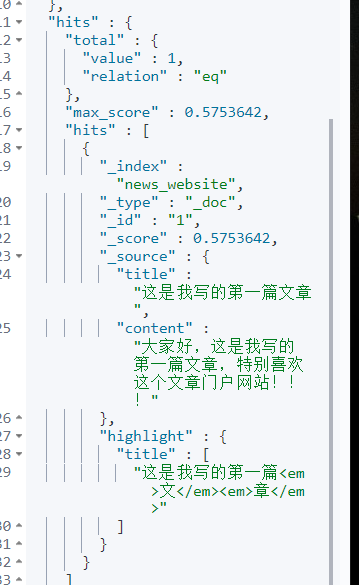
Note: the results may be different if the word splitters used are different. The default participle is used here;
GET /news_website/_doc/_search
 {
 "query": {
 "bool": {
 "should": [
 {
 "match": {
"title": "article"

 }
 },
 {
 "match": {
 "content": "article"
 }
 }
 ]
 }
 },
 "highlight": {
 "fields": {
 "title": {},
 "content": {}
 }
 }
 }
// The fields in highlight must be aligned one by one with the fields in query
Introduction to commonly used highlight
plain highlight, lucene highlight, default
posting highlight,index_options=offsets
(1) The performance is higher than plain highlight because there is no need to re segment the highlighted text
(2) Less disk consumption
PUT /news_website
{
"mappings": {
"_all": {
"title": {
"type": "text",
"analyzer": "ik_max_word"
},
"content": {
"type": "text",
"analyzer": "ik_max_word",
"index_options": "offsets"
}
}
}
}
PUT /news_website/_doc/1
{
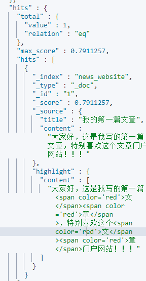
"title": "My first article",
"content": "Hello everyone, this is the first article I wrote. I especially like this article portal!!!"
}
GET /news_website/_doc/_search
{
"query": {
"match": {
"content": "article"
}
},
"highlight": {
"fields": {
"content": {}
}
}
}
To sum up, you can consider it according to your actual situation. Generally, plain highlight is enough. There is no need to make other additional settings. If you have high performance requirements for highlighting, you can try to enable posting highlight
//Set the highlighted html tag. The default is the < EM > tag

GET /news_website/_doc/_search
{
 "query": {
 "match": {
 "content": "article"
 }
 },
 "highlight": {
 "pre_tags": ["<span color='red'>"],
 "post_tags": ["</span>"],
 "fields": {
 "content": {
 "type": "plain"
 }
 }
 }
}
//Highlight the settings for the clip fragment


GET /_search
 {
 "query" : {
 "match": { "content": "article" }
 },
 "highlight" : {
 "fields" : {
 "content" : {"fragment_size" : 150, "number_of_fragments" : 3 }
 }
 }
 }
//fragment_size: you need a Field value, for example, the length is 10000, but you can't display it on the page
//Set the length of the fragment text to be displayed. The default is 100
// number_of_fragments: you may have multiple fragments in your highlighted fragment text fragment. You can specify how many fragments to display
In depth aggregation search technology
Bucket: a data grouping for aggregate search. For example, the sales department has employees Zhang San and Li Si, and the development department has employees Wang Wu and Zhao Liu. The result of department grouping and aggregation is two buckets. There are Zhang San and Li Si in the bucket of the sales department and Wang Wu and Zhao Liu in the bucket of the development department.
metric: statistical analysis performed on a bucket data. As in the above case, the development department has two employees
There are two employees in the sales department, which is metric. Metric has a variety of statistics, such as summation, maximum, minimum, average, etc.
PUT /cars
{
"mappings": {
"properties": {
"price": {
"type": "long"
},
"color": {
"type": "keyword"
},
"brand": {
"type": "keyword"
},
"model": {
"type": "keyword"
},
"sold_date": {
"type": "date"
},
"remark" : {
"type" : "text"
}
}
}
}
POST /cars/_bulk
{ "index": {}}
{ "price" : 258000, "color" : "golden", "brand":"public", "model" : "MAGOTAN", "remark" : "Volkswagen mid-range car" }
{ "index": {}}
{ "price" : 123000, "color" : "golden", "brand":"public", "model" : "Volkswagen Sagitar","remark" : "Volkswagen divine vehicle" }
{ "index": {}}
{ "price" : 239800, "color" : "white", "brand":"sign", "model" : "Sign 508", "remark" : "Global market model of logo brand" }
{ "index": {}}
{ "price" : 148800, "color" : "white", "brand":"sign", "model" : "Sign 408", "remark" : "Relatively large compact car" }
{ "index": {}}
{ "price" : 1998000, "color" : "black", "brand":"public", "model" : "Volkswagen Phaeton","remark" : "Volkswagen's most painful car" }
{ "index": {}}
{ "price" : 218000, "color" : "gules", "brand":"audi", "model" : "audi A4", "remark" : "Petty bourgeoisie model" }
{ "index": {}}
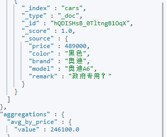
{ "price" : 489000, "color" : "black", "brand":"audi", "model" : "audi A6","remark" : "Government use?" }
{ "index": {}}
{ "price" : 1899000, "color" : "black", "brand":"audi", "model" : "audi A 8", "remark":"Very expensive big A6. . . " }
Aggregation operation
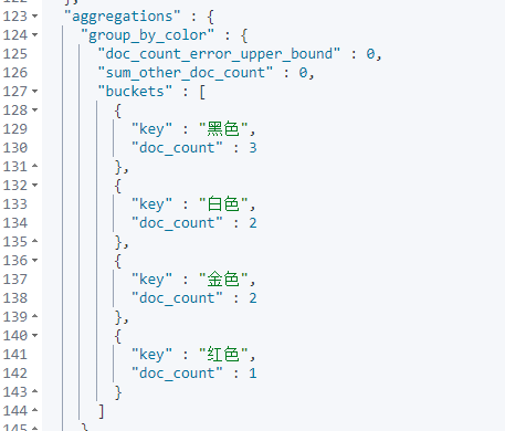
Only aggregate grouping is performed without complex aggregate statistics. In ES, the most basic aggregation is terms, which is equivalent to count in SQL.
In ES, grouping data is sorted by default, and DOC is used_ count data is arranged in descending order. Can use_ key metadata, which implements different sorting schemes according to the grouped field data, or_ count metadata, which implements different sorting schemes according to the grouped statistical values.
GET /cars/_search
{
  "aggs": {
    "group_by_color": {
      "terms": {
        "field": "color",
        "order": {
          "_count": "desc"
        }
      }
    }
  }
}
GET /cars/_search
{
  "aggs": {
    "group_by_color": {
      "terms": {
        "field": "color",
        "order": {
          "avg_by_price": "asc"
        }
      },
      "aggs": {
        "avg_by_price": {
          "avg": {
            "field": "price"
          }
        }
      }
    }
  }
}
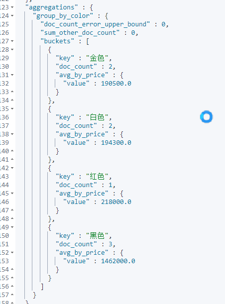
size can be set to 0, which means that the documents in ES are not returned, but only the data after ES aggregation, so as to improve the query speed. Of course, if you need these documents, you can also set them according to the actual situation
GET /cars/_search
{
  "size": 0,
  "aggs": {
    "group_by_color": {
      "terms": {
        "field": "color",
        "order": {
          "avg_by_price": "asc"
        }
      },
      "aggs": {
        "avg_by_price": {
          "avg": {
            "field": "price"
          }
        }
      }
    }
  }
}
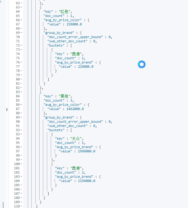
Count the average price of vehicles in different color s and brand s
First aggregate groups according to color, and then aggregate groups according to brand within the group. This operation can be called drill down analysis.
If there are many definitions of aggs, you will feel that the syntax format is chaotic. The aggs syntax format has a relatively fixed structure and simple definition: aggs can be nested or horizontally defined.
Nested definitions are called run in analysis. Horizontal definition is to tile multiple grouping methods.
GET /cars/_search
{
  "size": 0,
  "aggs": {
    "group_by_color": {
      "terms": {
        "field": "color",
        "order": {
          "avg_by_price_color": "asc"
        }
      },
      "aggs": {
        "avg_by_price_color": {
          "avg": {
            "field": "price"
          }
        },
        "group_by_brand": {
          "terms": {
            "field": "brand",
            "order": {
              "avg_by_price_brand": "desc"
            }
          },
          "aggs": {
            "avg_by_price_brand": {
              "avg": {
                "field": "price"
              }
            }
          }
        }
      }
    }
  }
}
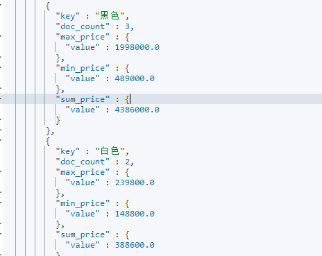
Count the maximum and minimum prices and total prices in different color s
GET /cars/_search
{
  "aggs": {
    "group_by_color": {
      "terms": {
        "field": "color"
      },
      "aggs": {
        "max_price": {
          "max": {
            "field": "price"
          }
        },
        "min_price": {
          "min": {
            "field": "price"
          }
        },
        "sum_price": {
          "sum": {
            "field": "price"
          }
        }
      }
    }
  }
}
In common business analysis, the most common types of aggregation analysis are statistical quantity, maximum, minimum and average,
Total, etc. It usually accounts for more than 60% of aggregation business, and even more than 85% of small projects.
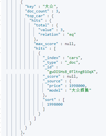
Make statistics on the models with the highest price among different brands of cars
After grouping, you may need to sort the data in the group and select the data with the highest ranking. So can
Using s to implement: Top_ top_ The attribute size in hithis represents the number of pieces of data in the group (the default is
10); sort represents the fields and sorting rules used in the group (the asc rule of _doc is used by default);
_ source represents those fields in the document included in the result (all fields are included by default).
GET cars/_search
{
  "size": 0,
  "aggs": {
    "group_by_brand": {
      "terms": {
        "field": "brand"
      },
      "aggs": {
        "top_car": {
          "top_hits": {
            "size": 1,
            "sort": [
              {
                "price": {
                  "order": "desc"
                }
              }
            ],
            "_source": {
              "includes": [
                "model",
                "price"
              ]
            }
          }
        }
      }
    }
  }
}
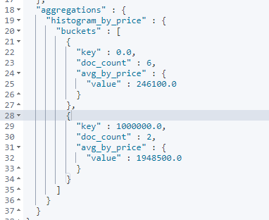
histogram interval statistics
histogram is similar to terms. It also performs bucket grouping. It realizes data interval grouping according to a field.
For example, take 1 million as a range to count the sales volume and average price of vehicles in different ranges. When using histogram aggregation, field specifies the price field price. The interval range is 1 million - interval: 1000000. At this time, ES will divide the price range into: [0, 1000000], [1000000000000], [2000000, 3000000), etc., and so on. While dividing the range, histogram will count the data quantity similar to terms, and the aggregated data in the group can be aggregated and analyzed again through nested aggs.
GET /cars/_search
{
  "size": 0,
  "aggs": {
    "histogram_by_price": {
      "histogram": {
        "field": "price",
        "interval": 1000000
      },
      "aggs": {
        "avg_by_price": {
          "avg": {
            "field": "price"
          }
        }
      }
    }
  }
}
date_histogram interval grouping
date_histogram can perform interval aggregation grouping for date type field s, such as monthly sales, annual sales, etc.
For example, take month as the unit to count the sales quantity and total sales amount of vehicles in different months. Date can be used at this time_ Histogram implements aggregation grouping, where field is used to specify the field used for aggregation grouping, Interval specifies the interval range (optional values are: year, quarter, month, week, day, hour, minute, second). Format specifies the date format. min_doc_count specifies the minimum document of each interval (if not specified, it is 0 by default. bucket grouping will also be displayed when there is no document in the interval range). extended_bounds specifies the start time and end time (if not specified, the range of the minimum value and the range of the maximum value of the date in the field are the start and end times by default).
GET /cars/_search
{
  "aggs": {
    "histogram_by_date": {
      "date_histogram": {
        "field": "sold_date",
        "calendar_interval": "month",
        "format": "yyyy‐MM‐dd",
        "min_doc_count": 1,
        "extended_bounds": {
          "min": "2021‐01‐01",
          "max": "2022‐12‐31"
        }
      },
      "aggs": {
        "sum_by_price": {
          "sum": {
            "field": "price"
          }
        }
      }
    }
  }
}
_global bucket
When aggregating statistics, it is sometimes necessary to compare partial data with overall data.
For example, make statistics on the average price of a brand of vehicles and the average price of all vehicles. Global is used to define a global
bucket, which ignores the query condition and retrieves all document s for corresponding aggregation statistics.
GET /cars/_search
{
  "size": 0,
  "query": {
    "match": {
      "brand": "public"
    }
  },
  "aggs": {
    "volkswagen_of_avg_price": {
      "avg": {
        "field": "price"
      }
    },
    "all_avg_price": {
      "global": {},
      "aggs": {
        "all_of_price": {
          "avg": {
            "field": "price"
          }
        }
      }
    }
  }
}
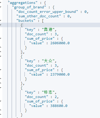
aggs+order
Sort aggregate statistics. For example, make statistics on the car sales and total sales of each brand, and arrange them in descending order of total sales.
GET /cars/_search
{
  "size": 0,
  "aggs": {
    "group_of_brand": {
      "terms": {
        "field": "brand",
        "order": {
          "sum_of_price": "desc"
        }
      },
      "aggs": {
        "sum_of_price": {
          "sum": {
            "field": "price"
          }
        }
      }
    }
  }
}
search+aggs
Aggregation is similar to the group by clause in SQL, and search is similar to the where clause in SQL. In ES, search and aggregations can be integrated to perform relatively more complex search statistics.
For example, make statistics on the sales and sales of a brand of vehicles in each quarter.
GET /cars/_search
{
  "query": {
    "match": {
      "brand": "public"
    }
  },
  "aggs": {
    "histogram_by_date": {
      "date_histogram": {
        "field": "sold_date",
        "calendar_interval": "quarter",
        "min_doc_count": 1
      },
      "aggs": {
        "sum_by_price": {
          "sum": {
            "field": "price"
          }
        }
      }
    }
  }
}
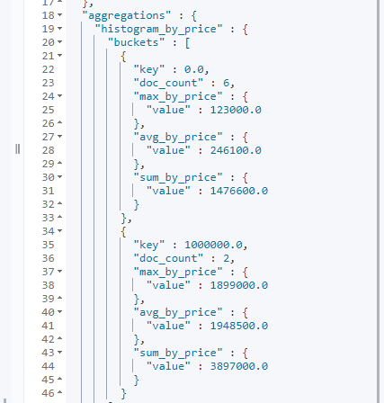
GET /cars/_search
{
  "size": 0,
  "aggs": {
    "histogram_by_price": {
      "histogram": {
        "field": "price",
        "interval": 1000000
      },
      "aggs": {
        "avg_by_price": {
          "avg": {
            "field": "price"
          }
        },
        "sum_by_price": {
          "sum": {
            "field": "price"
          }
        },
        "max_by_price": {
          "min": {
            "field": "price"
          }
        }
      }
    }
  }
}
filter+aggs
In ES, filter can also be combined with aggs to realize relatively complex filtering aggregation analysis.
For example, calculate the average price of vehicles between 100000 and 500000.
GET /cars/_search
{
  "query": {
    "constant_score": {
      "filter": {
        "range": {
          "price": {
            "gte": 100000,
            "lte": 500000
          }
        }
      }
    }
  },
  "aggs": {
    "avg_by_price": {
      "avg": {
        "field": "price"
      }
    }
  }
}