Research on traffic casualty accident prediction based on extended tecdat|R language Markov transformation model

Original link: http://tecdat.cn/?p=12227

Original source: Tuo end data tribal official account

abstract

This paper describes the analysis process of Markov transformation model in R language. Firstly, the simulation data set is modeled in detail. Next, the Markov transformation model is fitted to a real data set with discrete response variables. Different methods used to validate modeling of these data sets.

Simulation example

The sample data is a simulated data set that shows how to detect the existence of two different modes: the response variables in one mode are highly correlated, and the response in the other mode depends only on the exogenous variable x. The autocorrelation observations range from 1 to 100, 151 to 180, and 251 to 300. The real model of each scheme is:

The curve in Figure 1 shows that in the interval where there is no autocorrelation, the response variable y has a similar behavior to the covariate X. Fit the linear model to study how covariate x explains variable response y.

> summary(mod) 

Call:
lm(formula = y ~ x, data = example)

Residuals:

      Min 1Q Median 3Q Max

-2.8998 -0.8429 -0.0427 0.7420 4.0337

> plot(ts(example))

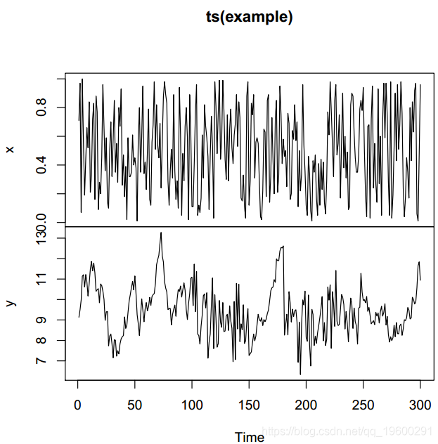
Figure 1: simulated data, y variable is the response variable

Coefficients:
Estimate Std. Error t value Pr(>|t|)

(Intercept)    9.0486    0.1398    64.709    < 2e-16 ***
x    0.8235    0.2423    3.398    0.00077 ***

Residual standard error: 1.208 on 298 degrees of freedom
Multiple R-squared: 0.03731, Adjusted R-squared: 0.03408
F-statistic: 11.55 on 1 and 298 DF, p-value: 0.0007701

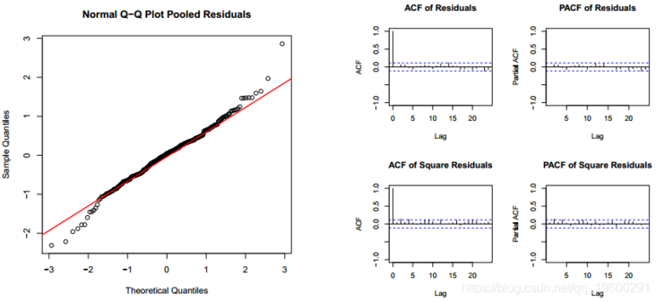
Covariates are really important, but the data behavior explained by the model is very bad. The linear model residual diagram in Figure 1 shows that they have strong autocorrelation. The diagnostic diagram of the residuals (Fig. 2) confirms that they do not appear to be white noise and have autocorrelation. Next, the autoregressive Markov transformation model (MSM-AR) is fitted to the data. The autoregressive part is set to 1. In order to indicate that all parameters can be different in two cycles, the transformation parameters are (sw) is set as a vector with four components. The last value when fitting the linear model is called the residual.

Standard deviation. There are options to control the estimation process, such as logical parameters that indicate whether process parallelization has been completed.

Markov Switching Model


AIC    BIC    logLik
637.0736 693.479 -312.5368
Coefficients:
Regime 1
\-\-\-\-\-\-\-\-\-
Estimate Std. Error t value    Pr(>|t|)
(Intercept)(S)    0.8417    0.3025    2.7825    0.005394 **
x(S)    -0.0533    0.1340 -0.3978    0.690778
y_1(S)    0.9208    0.0306 30.0915 < 2.2e-16 ***
\-\-\-
Signif. codes:    0    '***' 0.001    '**' 0.01    '*' 0.05    '.' 0.1    ' ' 1

Residual standard error: 0.5034675
Multiple R-squared: 0.8375

Standardized Residuals:
Min    Q1    Med    Q3    Max
-1.5153666657 -0.0906543311    0.0001873641    0.1656717256    1.2020898986
Regime 2
---------    Estimate Std. Error t value    Pr(>|t|)
(Intercept)(S)    8.6393    0.7244 11.9261 < 2.2e-16 ***
x(S)    1.8771    0.3107    6.0415 1.527e-09 ***
y_1(S)    -0.0569    0.0797 -0.7139    0.4753
\-\-\-
Signif. codes:    0    '***' 0.001    '**' 0.01    '*' 0.05    '.' 0.1    ' ' 1

Residual standard error: 0.9339683
Multiple R-squared: 0.2408
Standardized Residuals:
Min Q1 Med Q3 Max
-2.31102193 -0.03317756 0.01034139 0.04509105 2.85245598
Transition probabilities:
Regime 1 Regime 2
Regime 1 0.98499728 0.02290884
Regime 2 0.01500272 0.97709116

Model mod MSWM has a very significant state of covariance x, and in other cases, autocorrelation variables are also very important. Both have high values of R square. Finally, the transition probability matrix has a high value, which indicates that it is difficult to change from on state to another state. The model can perfectly detect the period of each state. The residuals look like white noise, and they are suitable for normal distribution. Moreover, the autocorrelation disappeared.

The graphical display has perfectly detected the cycle of each scheme.

> plot(mod.mswm,expl="x")

traffic accident

The traffic data include the daily number of traffic accidents, average daily temperature and daily precipitation in Spain in 2010. The purpose of the data is to study the relationship between the number of deaths and climatic conditions. Since there are different behaviors between weekend and weekday variables, we illustrate the use of generalized Markov transformation model in this case.
In this example, the response variable is the count variable. Therefore, we fit the Poisson generalized linear model.

> summary(model)
Call:
glm(formula = NDead ~ Temp + Prec, family = "poisson", data = traffic)

Deviance Residuals:

Min    1Q    Median    3Q    Max
-3.1571    -1.0676    -0.2119    0.8080    3.0629

Coefficients:
Estimate Std. Error z value Pr(>|z|)
(Intercept) 1.1638122 0.0808726 14.391 < 2e-16 ***
Temp 0.0225513 0.0041964 5.374 7.7e-08 ***
Prec 0.0002187 0.0001113 1.964 0.0495 *
\-\-\-
Signif. codes: 0 '***' 0.001 '**' 0.01 '*' 0.05 '.' 0.1 ' ' 1
(Dispersion parameter for poisson family taken to be 1)
Null deviance: 597.03 on 364 degrees of freedom
Residual deviance: 567.94 on 362 degrees of freedom
AIC: 1755.9
Number of Fisher Scoring iterations: 5

Next, a fitting Markov transformation model is used. In order to adapt to the generalized Markov transformation model, family parameters must be included, and glm has no standard deviation parameters, so sw parameters do not include its switching parameters.

> 
Markov Switching Model


AIC    BIC    logLik
1713.878 1772.676 -850.9388
Coefficients:
Regime 1
\-\-\-\-\-\-\-\-\-
Estimate Std. Error t value    Pr(>|t|)
(Intercept)(S)    0.7649    0.1755    4.3584    1.31e-05 ***
Temp(S)    0.0288    0.0082    3.5122 0.0004444 ***
Prec(S)    0.0002    0.0002    1.0000 0.3173105
\-\-\-
Signif. codes:    0    '***' 0.001    '**' 0.01    '*' 0.05    '.' 0.1    ' ' 1

Regime 2
\-\-\-\-\-\-\-\-\-
Estimate Std. Error t value Pr(>|t|)

(Intercept)(S)    1.5659    0.1576    9.9359    < 2e-16 ***
Temp(S)    0.0194    0.0080    2.4250    0.01531 *
Prec(S)    0.0004    0.0002    2.0000    0.04550 *
\-\-\-
Signif. codes:    0    '***' 0.001    '**' 0.01    '*' 0.05    '.' 0.1    ' ' 1

Transition probabilities:
Regime 1 Regime 2
Regime 1 0.7287732 0.4913893
Regime 2 0.2712268 0.5086107

Both states have significant covariates, but precipitation covariates are significant only in one of the two states.

Aproximate intervals for the coefficients. Level= 0.95
(Intercept):
Lower Estimation Upper
Regime 1 0.4208398 0.7648733 1.108907

Regime 2 1.2569375 1.5658582 1.874779
Temp:
Lower Estimation Upper
Regime 1 0.012728077 0.02884933 0.04497059
Regime 2 0.003708441 0.01939770 0.03508696
Prec:
Lower Estimation Upper
Regime 1 -1.832783e-04 0.0001846684 0.0005526152
Regime 2 -4.808567e-05 0.0004106061 0.0008692979

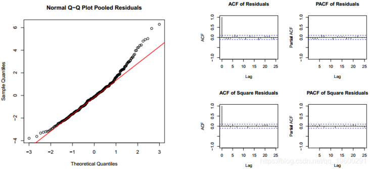
Since the model is an extension of the general linear model, the Pearson residual in the graph is calculated from the class object. The residual has the classical structure of white noise. The residuals are not autocorrelated, but they do not agree with the normal distribution. However, the normality of Pearson residuals is not the key condition for the verification of generalized linear models.