In previous articles, we introduced some knowledge based on genetic algorithm. This article will use genetic algorithm to process machine learning model and time series data.

Super parameter adjustment (TPOT)

Automatic machine learning (Auto ML) helps us find the most suitable model for prediction by automating the whole machine learning process. For machine learning model, Auto ML may more mean the adjustment and optimization of super parameters.

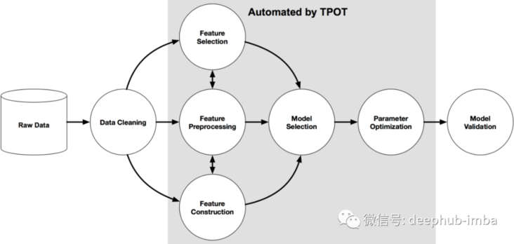
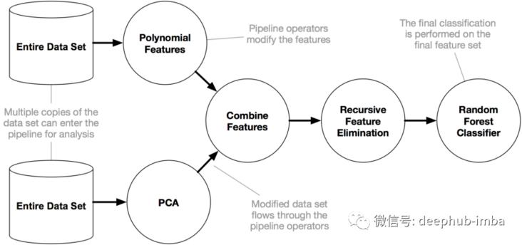
Here, we use a package named Tpot of python to operate. Tpot is based on scikit learn. Although it is still under development, its functions can help us understand these concepts. The following figure shows the working principle of Tpot:

from tpot import TPOTClassifier
from tpot import TPOTRegressormodel = TPOTClassifier(generations=100, population_size=100, offspring_size=None, mutation_rate=0.9, crossover_rate=0.1, scoring=None, cv=5, subsample=1.0, n_jobs=1, max_time_mins=None, max_eval_time_mins=5, random_state=None, config_dict=None, template=None, warm_start=False, memory=None, use_dask=False, periodic_checkpoint_folder=None, early_stop=None, verbosity=0, disable_update_check=False, log_file=None)

Through the above code, you can get a simple regression model, which is the default parameter list

generations=100, 
population_size=100, 
offspring_size=None  # Jeff notes this gets set to population_size
mutation_rate=0.9, 
crossover_rate=0.1, 
scoring="Accuracy",  # for Classification
cv=5, 
subsample=1.0, 
n_jobs=1,
max_time_mins=None, 
max_eval_time_mins=5,
random_state=None, 
config_dict=None,
warm_start=False, 
memory=None,
periodic_checkpoint_folder=None, 
early_stop=None
verbosity=0
disable_update_check=False

Let's see what super parameters can be adjusted:

generations : Number of iterations. The default value is 100.
population_size: The number of individuals retained in a genetically programmed population per generation. The default value is 100.
offspring_size: The number of offspring produced in each generation of genetic programming. The default value is 100.
mutation_rate: Mutation rate range of genetic programming algorithm[0.0, 1.0] . This parameter tells GP How many pipes does the algorithm apply random changes to each word iteration. The default value is 0.9
crossover_rate: Genetic programming algorithm, crossover rate, range[0.0, 1.0] . This parameter tells the genetic programming algorithm how many pipelines to "cultivate" in each generation.
scoring: Functions used to evaluate the problem, such as accuracy, average accuracy roc_auc,Recall rate, etc. The default is accuracy.
cv: Cross validation strategy used when evaluating pipelines. The default value is 5.
random_state: TPOT The seed of the pseudo-random number generator used in. Use this parameter to ensure operation TPOT The same random seeds are used to get the same results.
n_jobs: = -1 Multiple CPU Run on the kernel to speed up tpot Process.
period_checkpoint_folder: "any_string"，The evolution of the model can be observed while the training score is improved.

mutation_rate + crossover_rate cannot exceed 1.0.

Next, we use Tpot and sklearn to train the model.

from pandas import read_csv
from sklearn.preprocessing import LabelEncoder
from sklearn.model_selection import RepeatedStratifiedKFold
from tpot import TPOTClassifier

dataframe = read_csv('sonar.csv')
#define X and y 
data = dataframe.values
X, y = data[:, :-1], data[:, -1]

# minimally prepare dataset
X = X.astype('float32')
y = LabelEncoder().fit_transform(y.astype('str'))

#split the dataset
from sklearn.model_selection import train_test_split
X_train, X_test, y_train, y_test = train_test_split(X, y, test_size = 0.2, random_state = 0)

# define cross validation 
cv = RepeatedStratifiedKFold(n_splits=10, n_repeats=3, random_state=1)

Now let's run TPOTClassifier to optimize the super parameters

#initialize the classifier
model = TPOTClassifier(generations=5, population_size=50,max_time_mins= 2,cv=cv, scoring='accuracy', verbosity=2, random_state=1, n_jobs=-1)
model.fit(X_train, y_train)

#export the best model
model.export('tpot_best_model.py')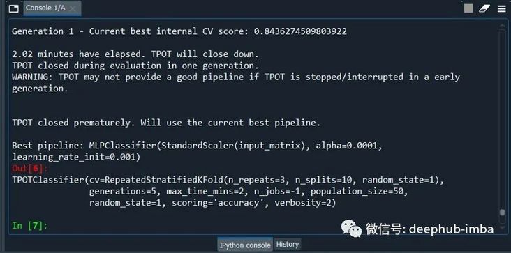

The last sentence of code saves the model in py file, you can import directly after using. Because the biggest problem for AutoML is the training time, in order to save time, population_size,max_time_mins equivalence uses the minimum setting.

Now let's open the file tpot_best_model.py, look at the content:

import numpy as np
import pandas as pd
from sklearn.linear_model import RidgeCV
from sklearn.model_selection import train_test_split
from sklearn.pipeline import make_pipeline
from sklearn.preprocessing import PolynomialFeatures
from tpot.export_utils import set_param_recursive

# NOTE: Make sure that the outcome column is labeled 'target' in the data file
tpot_data = pd.read_csv('PATH/TO/DATA/FILE', sep='COLUMN_SEPARATOR', dtype=np.float64)
features = tpot_data.drop('target', axis=1)
training_features, testing_features, training_target, testing_target = \
            train_test_split(features, tpot_data['target'], random_state=1)

# Average CV score on the training set was: -29.099695845082277
exported_pipeline = make_pipeline(
    PolynomialFeatures(degree=2, include_bias=False, interaction_only=False),
    RidgeCV()
)

# Fix random state for all the steps in exported pipeline
set_param_recursive(exported_pipeline.steps, 'random_state', 1)

exported_pipeline.fit(training_features, training_target)
results = exported_pipeline.predict(testing_features)

If you want to make a prediction, use the following code

yhat = exported_pipeline.predict(new_data)

The above is the super parameter optimization method of genetic algorithm in AutoML / machine learning. Genetic algorithm is inspired by Darwin's natural selection process and is used in computer science to find optimization search. In short, genetic algorithm consists of three common behaviors: selection, crossover and mutation

Let's see how it helps the model dealing with time series

Time series data modeling (AutoTS)

In Python, there is a package called AutoTS that can process time series data. Let's start with it

#AutoTS
from autots import AutoTS
from autots.models.model_list import model_lists
print(model_lists)

There are many different types of time series models in autots. Based on these algorithms, he finds the optimal model through the optimization of genetic algorithm.

Now let's load the data.

#default data
from autots.datasets import load_monthly
#data was in long format
df_long = load_monthly(long=True)

Initialize AutoTS with different parameters

model = AutoTS(
    forecast_length=3,
    frequency='infer',
    ensemble='simple',
    max_generations=5,
    num_validations=2,
)
model = model.fit(df_long, date_col='datetime', value_col='value', id_col='series_id')
#help(AutoTS)

This step takes a long time because it must go through multiple algorithm iterations.

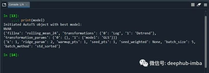
print(model)

We can also view the model accuracy score

#accuracy score
model.results()
#aggregated from cross validation
validation_results = model.results("validation")

From the list of model accuracy scores, you can also see the column "Ensemble" highlighted above. Its low precision verifies a theory that Ensemble always performs better. This statement is incorrect.

If you find the best model, you can make a prediction.

prediction = model.predict()
forecasts_df = prediction.forecast
upper_forecasts_df = prediction.upper_forecast
lower_forecasts_df = prediction.lower_forecast
#or
forecasts_df1 = prediction.long_form_results()
upper_forecasts_df1 = prediction.long_form_results()
lower_forecasts_df1 = prediction.long_form_results()

The default method is to use all models provided by AutoTs for training. If we want to execute on some model lists and set different weights for a feature, we need some custom configurations.

First, read the data

from autots import AutoTS
from autots.datasets import load_hourlydf_wide = load_hourly(long=False)

# here we care most about traffic volume, all other series assumed to be weight of 1
weights_hourly = {'traffic_volume': 20}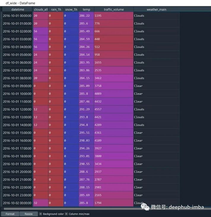

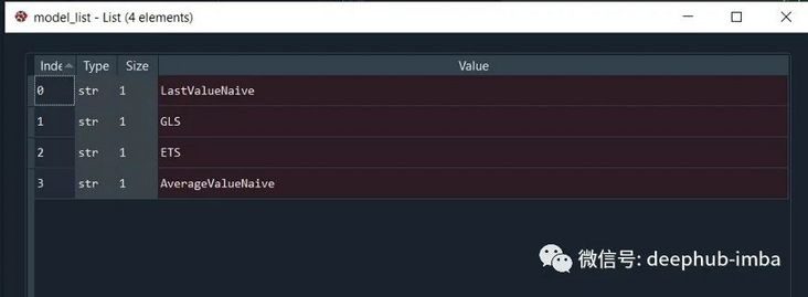
Define Model List:

model_list = [
    'LastValueNaive',
    'GLS',
    'ETS',
    'AverageValueNaive',
]

model = AutoTS(
    forecast_length=49,
    frequency='infer',
    prediction_interval=0.95,
    ensemble=['simple', 'horizontal-min'],
    max_generations=5,
    num_validations=2,
    validation_method='seasonal 168',
    model_list=model_list,
    transformer_list='all',
    models_to_validate=0.2,
    drop_most_recent=1,
    n_jobs='auto',
)

Define weights when fitting models with data:

model = model.fit(
    df_wide,
    weights=weights_hourly,
)

prediction = model.predict()
forecasts_df = prediction.forecast

This is done, which is very simple for use

Related resources

The following are the documentation for the two python packages:

https://winedarksea.github.io...

http://epistasislab.github.io...

Finally, if you are interested in participating in the Kaggle competition, please write to me and invite you to join the Kaggle competition exchange group